Page Summary
-
This content provides definitions for fundamental machine learning terms, including concepts related to models, training, features, and evaluation.
-
It covers a broad range of topics such as supervised/unsupervised learning, neural networks, regularization, loss functions, and specific algorithms like linear/logistic regression.
-
The glossary aims to equip beginners with essential vocabulary for comprehending core machine learning principles.
-
Various practical considerations like data preprocessing techniques (normalization, bucketing), dealing with imbalanced datasets, and preventing overfitting are also addressed.
-
The content serves as a foundational resource for individuals starting their machine learning journey, offering clear explanations and illustrations of key concepts.
This page contains ML Fundamentals glossary terms. For all glossary terms, click here.
A
accuracy
The number of correct classification predictions divided by the total number of predictions. That is:
For example, a model that made 40 correct predictions and 10 incorrect predictions would have an accuracy of:
Binary classification provides specific names for the different categories of correct predictions and incorrect predictions. So, the accuracy formula for binary classification is as follows:
where:
- TP is the number of true positives (correct predictions).
- TN is the number of true negatives (correct predictions).
- FP is the number of false positives (incorrect predictions).
- FN is the number of false negatives (incorrect predictions).
Compare and contrast accuracy with precision and recall.
See Classification: Accuracy, recall, precision and related metrics in Machine Learning Crash Course for more information.
activation function
A function that enables neural networks to learn nonlinear (complex) relationships between features and the label.
Popular activation functions include:
The plots of activation functions are never single straight lines. For example, the plot of the ReLU activation function consists of two straight lines:

A plot of the sigmoid activation function looks as follows:

See Neural networks: Activation functions in Machine Learning Crash Course for more information.
artificial intelligence
A non-human program or model that can solve sophisticated tasks. For example, a program or model that translates text or a program or model that identifies diseases from radiologic images both exhibit artificial intelligence.
Formally, machine learning is a sub-field of artificial intelligence. However, in recent years, some organizations have begun using the terms artificial intelligence and machine learning interchangeably.
AUC (Area under the ROC curve)
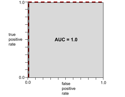
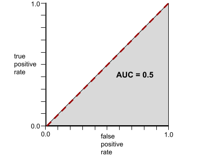
A number between 0.0 and 1.0 representing a binary classification model's ability to separate positive classes from negative classes. The closer the AUC is to 1.0, the better the model's ability to separate classes from each other.
For example, the following illustration shows a classification model that separates positive classes (green ovals) from negative classes (purple rectangles) perfectly. This unrealistically perfect model has an AUC of 1.0:

Conversely, the following illustration shows the results for a classification model that generated random results. This model has an AUC of 0.5:

Yes, the preceding model has an AUC of 0.5, not 0.0.
Most models are somewhere between the two extremes. For instance, the following model separates positives from negatives somewhat, and therefore has an AUC somewhere between 0.5 and 1.0:

AUC ignores any value you set for classification threshold. Instead, AUC considers all possible classification thresholds.
See Classification: ROC and AUC in Machine Learning Crash Course for more information.
B
backpropagation
The algorithm that implements gradient descent in neural networks.
Training a neural network involves many iterations of the following two-pass cycle:
- During the forward pass, the system processes a batch of examples to yield prediction(s). The system compares each prediction to each label value. The difference between the prediction and the label value is the loss for that example. The system aggregates the losses for all the examples to compute the total loss for the current batch.
- During the backward pass (backpropagation), the system reduces loss by adjusting the weights of all the neurons in all the hidden layer(s).
Neural networks often contain many neurons across many hidden layers. Each of those neurons contribute to the overall loss in different ways. Backpropagation determines whether to increase or decrease the weights applied to particular neurons.
The learning rate is a multiplier that controls the degree to which each backward pass increases or decreases each weight. A large learning rate will increase or decrease each weight more than a small learning rate.
In calculus terms, backpropagation implements the chain rule. from calculus. That is, backpropagation calculates the partial derivative of the error with respect to each parameter.
Years ago, ML practitioners had to write code to implement backpropagation. Modern ML APIs like Keras now implement backpropagation for you. Phew!
See Neural networks in Machine Learning Crash Course for more information.
batch
The set of examples used in one training iteration. The batch size determines the number of examples in a batch.
See epoch for an explanation of how a batch relates to an epoch.
See Linear regression: Hyperparameters in Machine Learning Crash Course for more information.
batch size
The number of examples in a batch. For instance, if the batch size is 100, then the model processes 100 examples per iteration.
The following are popular batch size strategies:
- Stochastic Gradient Descent (SGD), in which the batch size is 1.
- Full batch, in which the batch size is the number of examples in the entire training set. For instance, if the training set contains a million examples, then the batch size would be a million examples. Full batch is usually an inefficient strategy.
- mini-batch in which the batch size is usually between 10 and 1000. Mini-batch is usually the most efficient strategy.
See the following for more information:
- Production ML systems: Static versus dynamic inference in Machine Learning Crash Course.
- Deep Learning Tuning Playbook.
bias (ethics/fairness)
1. Stereotyping, prejudice or favoritism towards some things, people, or groups over others. These biases can affect collection and interpretation of data, the design of a system, and how users interact with a system. Forms of this type of bias include:
- automation bias
- confirmation bias
- experimenter's bias
- group attribution bias
- implicit bias
- in-group bias
- out-group homogeneity bias
2. Systematic error introduced by a sampling or reporting procedure. Forms of this type of bias include:
Not to be confused with the bias term in machine learning models or prediction bias.
See Fairness: Types of bias in Machine Learning Crash Course for more information.
bias (math) or bias term
An intercept or offset from an origin. Bias is a parameter in machine learning models, which is symbolized by either of the following:
- b
- w0
For example, bias is the b in the following formula:
In a simple two-dimensional line, bias just means "y-intercept." For example, the bias of the line in the following illustration is 2.
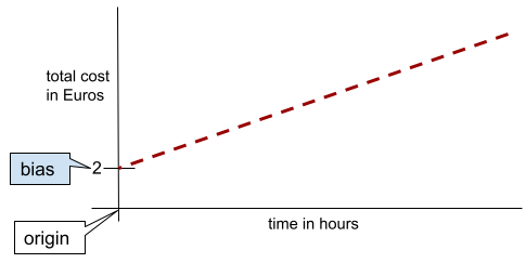
Bias exists because not all models start from the origin (0,0). For example, suppose an amusement park costs 2 Euros to enter and an additional 0.5 Euro for every hour a customer stays. Therefore, a model mapping the total cost has a bias of 2 because the lowest cost is 2 Euros.
Bias is not to be confused with bias in ethics and fairness or prediction bias.
See Linear Regression in Machine Learning Crash Course for more information.
binary classification
A type of classification task that predicts one of two mutually exclusive classes:
- the positive class
- the negative class
For example, the following two machine learning models each perform binary classification:
- A model that determines whether email messages are spam (the positive class) or not spam (the negative class).
- A model that evaluates medical symptoms to determine whether a person has a particular disease (the positive class) or doesn't have that disease (the negative class).
Contrast with multi-class classification.
See also logistic regression and classification threshold.
See Classification in Machine Learning Crash Course for more information.
bucketing
Converting a single feature into multiple binary features called buckets or bins, typically based on a value range. The chopped feature is typically a continuous feature.
For example, instead of representing temperature as a single continuous floating-point feature, you could chop ranges of temperatures into discrete buckets, such as:
- <= 10 degrees Celsius would be the "cold" bucket.
- 11 - 24 degrees Celsius would be the "temperate" bucket.
- >= 25 degrees Celsius would be the "warm" bucket.
The model will treat every value in the same bucket identically. For
example, the values 13 and 22 are both in the temperate bucket, so the
model treats the two values identically.
See Numerical data: Binning in Machine Learning Crash Course for more information.
C
categorical data
Features having a specific set of possible values. For example,
consider a categorical feature named traffic-light-state, which can only
have one of the following three possible values:
redyellowgreen
By representing traffic-light-state as a categorical feature,
a model can learn the
differing impacts of red, green, and yellow on driver behavior.
Categorical features are sometimes called discrete features.
Contrast with numerical data.
See Working with categorical data in Machine Learning Crash Course for more information.
class
A category that a label can belong to. For example:
- In a binary classification model that detects spam, the two classes might be spam and not spam.
- In a multi-class classification model that identifies dog breeds, the classes might be poodle, beagle, pug, and so on.
A classification model predicts a class. In contrast, a regression model predicts a number rather than a class.
See Classification in Machine Learning Crash Course for more information.
classification model
A model whose prediction is a class. For example, the following are all classification models:
- A model that predicts an input sentence's language (French? Spanish? Italian?).
- A model that predicts tree species (Maple? Oak? Baobab?).
- A model that predicts the positive or negative class for a particular medical condition.
In contrast, regression models predict numbers rather than classes.
Two common types of classification models are:
classification threshold
In a binary classification, a number between 0 and 1 that converts the raw output of a logistic regression model into a prediction of either the positive class or the negative class. Note that the classification threshold is a value that a human chooses, not a value chosen by model training.
A logistic regression model outputs a raw value between 0 and 1. Then:
- If this raw value is greater than the classification threshold, then the positive class is predicted.
- If this raw value is less than the classification threshold, then the negative class is predicted.
For example, suppose the classification threshold is 0.8. If the raw value is 0.9, then the model predicts the positive class. If the raw value is 0.7, then the model predicts the negative class.
The choice of classification threshold strongly influences the number of false positives and false negatives.
See Thresholds and the confusion matrix in Machine Learning Crash Course for more information.
classifier
A casual term for a classification model.
class-imbalanced dataset
A dataset for a classification in which the total number of labels of each class differs significantly. For example, consider a binary classification dataset whose two labels are divided as follows:
- 1,000,000 negative labels
- 10 positive labels
The ratio of negative to positive labels is 100,000 to 1, so this is a class-imbalanced dataset.
In contrast, the following dataset is class-balanced because the ratio of negative labels to positive labels is relatively close to 1:
- 517 negative labels
- 483 positive labels
Multi-class datasets can also be class-imbalanced. For example, the following multi-class classification dataset is also class-imbalanced because one label has far more examples than the other two:
- 1,000,000 labels with class "green"
- 200 labels with class "purple"
- 350 labels with class "orange"
Training class-imbalanced datasets can present special challenges. See Imbalanced datasets in Machine Learning Crash Course for details.
See also entropy, majority class, and minority class.
clipping
A technique for handling outliers by doing either or both of the following:
- Reducing feature values that are greater than a maximum threshold down to that maximum threshold.
- Increasing feature values that are less than a minimum threshold up to that minimum threshold.
For example, suppose that <0.5% of values for a particular feature fall outside the range 40–60. In this case, you could do the following:
- Clip all values over 60 (the maximum threshold) to be exactly 60.
- Clip all values under 40 (the minimum threshold) to be exactly 40.
Outliers can damage models, sometimes causing weights to overflow during training. Some outliers can also dramatically spoil metrics like accuracy. Clipping is a common technique to limit the damage.
Gradient clipping forces gradient values within a designated range during training.
See Numerical data: Normalization in Machine Learning Crash Course for more information.
confusion matrix
An NxN table that summarizes the number of correct and incorrect predictions that a classification model made. For example, consider the following confusion matrix for a binary classification model:
| Tumor (predicted) | Non-Tumor (predicted) | |
|---|---|---|
| Tumor (ground truth) | 18 (TP) | 1 (FN) |
| Non-Tumor (ground truth) | 6 (FP) | 452 (TN) |
The preceding confusion matrix shows the following:
- Of the 19 predictions in which ground truth was Tumor, the model correctly classified 18 and incorrectly classified 1.
- Of the 458 predictions in which ground truth was Non-Tumor, the model correctly classified 452 and incorrectly classified 6.
The confusion matrix for a multi-class classification problem can help you identify patterns of mistakes. For example, consider the following confusion matrix for a 3-class multi-class classification model that categorizes three different iris types (Virginica, Versicolor, and Setosa). When the ground truth was Virginica, the confusion matrix shows that the model was far more likely to mistakenly predict Versicolor than Setosa:
| Setosa (predicted) | Versicolor (predicted) | Virginica (predicted) | |
|---|---|---|---|
| Setosa (ground truth) | 88 | 12 | 0 |
| Versicolor (ground truth) | 6 | 141 | 7 |
| Virginica (ground truth) | 2 | 27 | 109 |
As yet another example, a confusion matrix could reveal that a model trained to recognize handwritten digits tends to mistakenly predict 9 instead of 4, or mistakenly predict 1 instead of 7.
Confusion matrixes contain sufficient information to calculate a variety of performance metrics, including precision and recall.
continuous feature
A floating-point feature with an infinite range of possible values, such as temperature or weight.
Contrast with discrete feature.
convergence
A state reached when loss values change very little or not at all with each iteration. For example, the following loss curve suggests convergence at around 700 iterations:
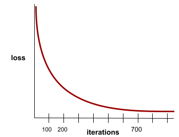
A model converges when additional training won't improve the model.
In deep learning, loss values sometimes stay constant or nearly so for many iterations before finally descending. During a long period of constant loss values, you may temporarily get a false sense of convergence.
See also early stopping.
See Model convergence and loss curves in Machine Learning Crash Course for more information.
D
DataFrame
A popular pandas data type for representing datasets in memory.
A DataFrame is analogous to a table or a spreadsheet. Each column of a DataFrame has a name (a header), and each row is identified by a unique number.
Each column in a DataFrame is structured like a 2D array, except that each column can be assigned its own data type.
See also the official pandas.DataFrame reference page.
data set or dataset
A collection of raw data, commonly (but not exclusively) organized in one of the following formats:
- a spreadsheet
- a file in CSV (comma-separated values) format
deep model
A neural network containing more than one hidden layer.
A deep model is also called a deep neural network.
Contrast with wide model.
dense feature
A feature in which most or all values are nonzero, typically a Tensor of floating-point values. For example, the following 10-element Tensor is dense because 9 of its values are nonzero:
| 8 | 3 | 7 | 5 | 2 | 4 | 0 | 4 | 9 | 6 |
Contrast with sparse feature.
depth
The sum of the following in a neural network:
- the number of hidden layers
- the number of output layers, which is typically 1
- the number of any embedding layers
For example, a neural network with five hidden layers and one output layer has a depth of 6.
Notice that the input layer doesn't influence depth.
discrete feature
A feature with a finite set of possible values. For example, a feature whose values may only be animal, vegetable, or mineral is a discrete (or categorical) feature.
Contrast with continuous feature.
dynamic
Something done frequently or continuously. The terms dynamic and online are synonyms in machine learning. The following are common uses of dynamic and online in machine learning:
- A dynamic model (or online model) is a model that is retrained frequently or continuously.
- Dynamic training (or online training) is the process of training frequently or continuously.
- Dynamic inference (or online inference) is the process of generating predictions on demand.
dynamic model
A model that is frequently (maybe even continuously) retrained. A dynamic model is a "lifelong learner" that constantly adapts to evolving data. A dynamic model is also known as an online model.
Contrast with static model.
E
early stopping
A method for regularization that involves ending training before training loss finishes decreasing. In early stopping, you intentionally stop training the model when the loss on a validation dataset starts to increase; that is, when generalization performance worsens.
Contrast with early exit.
embedding layer
A special hidden layer that trains on a high-dimensional categorical feature to gradually learn a lower dimension embedding vector. An embedding layer enables a neural network to train far more efficiently than training just on the high-dimensional categorical feature.
For example, Earth currently supports about 73,000 tree species. Suppose
tree species is a feature in your model, so your model's
input layer includes a one-hot vector 73,000
elements long.
For example, perhaps baobab would be represented something like this:

A 73,000-element array is very long. If you don't add an embedding layer to the model, training is going to be very time consuming due to multiplying 72,999 zeros. Perhaps you pick the embedding layer to consist of 12 dimensions. Consequently, the embedding layer will gradually learn a new embedding vector for each tree species.
In certain situations, hashing is a reasonable alternative to an embedding layer.
See Embeddings in Machine Learning Crash Course for more information.
epoch
A full training pass over the entire training set such that each example has been processed once.
An epoch represents N/batch size
training iterations, where N is the
total number of examples.
For instance, suppose the following:
- The dataset consists of 1,000 examples.
- The batch size is 50 examples.
Therefore, a single epoch requires 20 iterations:
1 epoch = (N/batch size) = (1,000 / 50) = 20 iterations
See Linear regression: Hyperparameters in Machine Learning Crash Course for more information.
example
The values of one row of features and possibly a label. Examples in supervised learning fall into two general categories:
- A labeled example consists of one or more features and a label. Labeled examples are used during training.
- An unlabeled example consists of one or more features but no label. Unlabeled examples are used during inference.
For instance, suppose you are training a model to determine the influence of weather conditions on student test scores. Here are three labeled examples:
| Features | Label | ||
|---|---|---|---|
| Temperature | Humidity | Pressure | Test score |
| 15 | 47 | 998 | Good |
| 19 | 34 | 1020 | Excellent |
| 18 | 92 | 1012 | Poor |
Here are three unlabeled examples:
| Temperature | Humidity | Pressure | |
|---|---|---|---|
| 12 | 62 | 1014 | |
| 21 | 47 | 1017 | |
| 19 | 41 | 1021 |
The row of a dataset is typically the raw source for an example. That is, an example typically consists of a subset of the columns in the dataset. Furthermore, the features in an example can also include synthetic features, such as feature crosses.
See Supervised Learning in the Introduction to Machine Learning course for more information.
F
false negative (FN)
An example in which the model mistakenly predicts the negative class. For example, the model predicts that a particular email message is not spam (the negative class), but that email message actually is spam.
false positive (FP)
An example in which the model mistakenly predicts the positive class. For example, the model predicts that a particular email message is spam (the positive class), but that email message is actually not spam.
See Thresholds and the confusion matrix in Machine Learning Crash Course for more information.
false positive rate (FPR)
The proportion of actual negative examples for which the model mistakenly predicted the positive class. The following formula calculates the false positive rate:
The false positive rate is the x-axis in an ROC curve.
See Classification: ROC and AUC in Machine Learning Crash Course for more information.
feature
An input variable to a machine learning model. An example consists of one or more features. For instance, suppose you are training a model to determine the influence of weather conditions on student test scores. The following table shows three examples, each of which contains three features and one label:
| Features | Label | ||
|---|---|---|---|
| Temperature | Humidity | Pressure | Test score |
| 15 | 47 | 998 | 92 |
| 19 | 34 | 1020 | 84 |
| 18 | 92 | 1012 | 87 |
Contrast with label.
See Supervised Learning in the Introduction to Machine Learning course for more information.
feature cross
A synthetic feature formed by "crossing" categorical or bucketed features.
For example, consider a "mood forecasting" model that represents temperature in one of the following four buckets:
freezingchillytemperatewarm
And represents wind speed in one of the following three buckets:
stilllightwindy
Without feature crosses, the linear model trains independently on each of the
preceding seven various buckets. So, the model trains on, for example,
freezing independently of the training on, for example,
windy.
Alternatively, you could create a feature cross of temperature and wind speed. This synthetic feature would have the following 12 possible values:
freezing-stillfreezing-lightfreezing-windychilly-stillchilly-lightchilly-windytemperate-stilltemperate-lighttemperate-windywarm-stillwarm-lightwarm-windy
Thanks to feature crosses, the model can learn mood differences
between a freezing-windy day and a freezing-still day.
If you create a synthetic feature from two features that each have a lot of different buckets, the resulting feature cross will have a huge number of possible combinations. For example, if one feature has 1,000 buckets and the other feature has 2,000 buckets, the resulting feature cross has 2,000,000 buckets.
Formally, a cross is a Cartesian product.
Feature crosses are mostly used with linear models and are rarely used with neural networks.
See Categorical data: Feature crosses in Machine Learning Crash Course for more information.
feature engineering
A process that involves the following steps:
- Determining which features might be useful in training a model.
- Converting raw data from the dataset into efficient versions of those features.
For example, you might determine that temperature might be a useful
feature. Then, you might experiment with bucketing
to optimize what the model can learn from different temperature ranges.
Feature engineering is sometimes called feature extraction or featurization.
See Numerical data: How a model ingests data using feature vectors in Machine Learning Crash Course for more information.
feature set
The group of features your machine learning model trains on. For example, a simple feature set for a model that predicts housing prices might consist of postal code, property size, and property condition.
feature vector
The array of feature values comprising an example. The feature vector is input during training and during inference. For example, the feature vector for a model with two discrete features might be:
[0.92, 0.56]
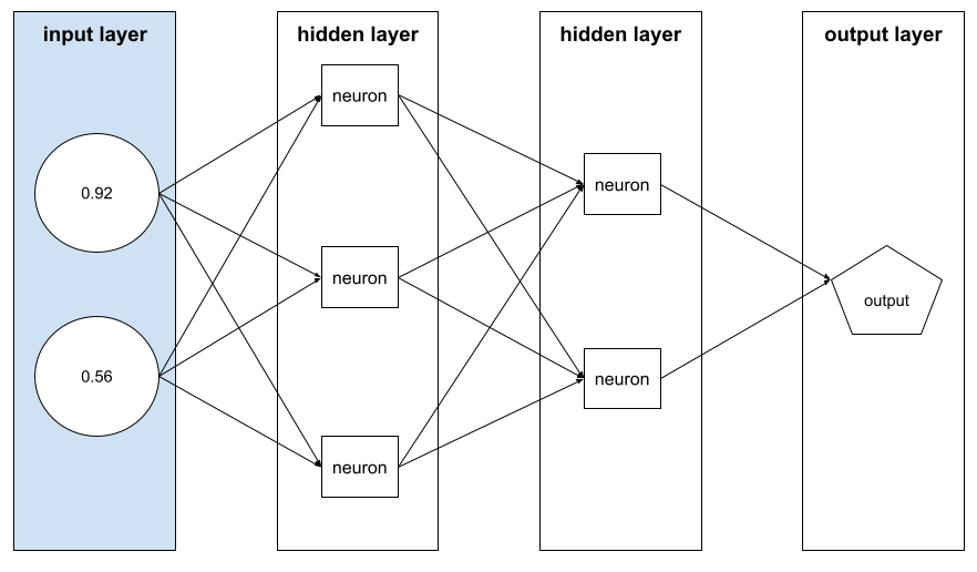
Each example supplies different values for the feature vector, so the feature vector for the next example could be something like:
[0.73, 0.49]
Feature engineering determines how to represent features in the feature vector. For example, a binary categorical feature with five possible values might be represented with one-hot encoding. In this case, the portion of the feature vector for a particular example would consist of four zeroes and a single 1.0 in the third position, as follows:
[0.0, 0.0, 1.0, 0.0, 0.0]
As another example, suppose your model consists of three features:
- a binary categorical feature with five possible values represented with
one-hot encoding; for example:
[0.0, 1.0, 0.0, 0.0, 0.0] - another binary categorical feature with three possible values represented
with one-hot encoding; for example:
[0.0, 0.0, 1.0] - a floating-point feature; for example:
8.3.
In this case, the feature vector for each example would be represented by nine values. Given the example values in the preceding list, the feature vector would be:
0.0
1.0
0.0
0.0
0.0
0.0
0.0
1.0
8.3
See Numerical data: How a model ingests data using feature vectors in Machine Learning Crash Course for more information.
feedback loop
In machine learning, a situation in which a model's predictions influence the training data for the same model or another model. For example, a model that recommends movies will influence the movies that people see, which will then influence subsequent movie recommendation models.
See Production ML systems: Questions to ask in Machine Learning Crash Course for more information.
G
generalization
A model's ability to make correct predictions on new, previously unseen data. A model that can generalize is the opposite of a model that is overfitting.
See Generalization in Machine Learning Crash Course for more information.
generalization curve
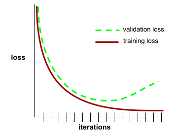
A plot of both training loss and validation loss as a function of the number of iterations.
A generalization curve can help you detect possible overfitting. For example, the following generalization curve suggests overfitting because validation loss ultimately becomes significantly higher than training loss.
See Generalization in Machine Learning Crash Course for more information.
gradient descent
A mathematical technique to minimize loss. Gradient descent iteratively adjusts weights and biases, gradually finding the best combination to minimize loss.
Gradient descent is older—much, much older—than machine learning.
See the Linear regression: Gradient descent in Machine Learning Crash Course for more information.
ground truth
Reality.
The thing that actually happened.
For example, consider a binary classification model that predicts whether a student in their first year of university will graduate within six years. Ground truth for this model is whether or not that student actually graduated within six years.
H
hidden layer
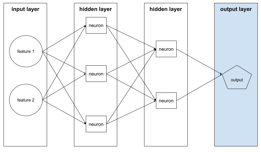
A layer in a neural network between the input layer (the features) and the output layer (the prediction). Each hidden layer consists of one or more neurons. For example, the following neural network contains two hidden layers, the first with three neurons and the second with two neurons:
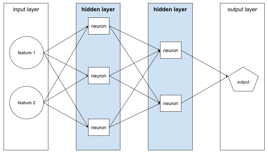
A deep neural network contains more than one hidden layer. For example, the preceding illustration is a deep neural network because the model contains two hidden layers.
See Neural networks: Nodes and hidden layers in Machine Learning Crash Course for more information.
hyperparameter
The variables that you or a hyperparameter tuning service adjust during successive runs of training a model. For example, learning rate is a hyperparameter. You could set the learning rate to 0.01 before one training session. If you determine that 0.01 is too high, you could perhaps set the learning rate to 0.003 for the next training session.
In contrast, parameters are the various weights and bias that the model learns during training.
See Linear regression: Hyperparameters in Machine Learning Crash Course for more information.
I
independently and identically distributed (i.i.d)
Data drawn from a distribution that doesn't change, and where each value drawn doesn't depend on values that have been drawn previously. An i.i.d. is the ideal gas of machine learning—a useful mathematical construct but almost never exactly found in the real world. For example, the distribution of visitors to a web page may be i.i.d. over a brief window of time; that is, the distribution doesn't change during that brief window and one person's visit is generally independent of another's visit. However, if you expand that window of time, seasonal differences in the web page's visitors may appear.
See also nonstationarity.
inference
In traditional machine learning, the process of making predictions by applying a trained model to unlabeled examples. See Supervised Learning in the Intro to ML course to learn more.
In large language models, inference is the process of using a trained model to generate a response to an input prompt.
Inference has a somewhat different meaning in statistics. See the Wikipedia article on statistical inference for details.
input layer
The layer of a neural network that holds the feature vector. That is, the input layer provides examples for training or inference. For example, the input layer in the following neural network consists of two features:

interpretability
The ability to explain or to present an ML model's reasoning in understandable terms to a human.
Most linear regression models, for example, are highly interpretable. (You merely need to look at the trained weights for each feature.) Decision forests are also highly interpretable. Some models, however, require sophisticated visualization to become interpretable.
You can use the Learning Interpretability Tool (LIT) to interpret ML models.
iteration
A single update of a model's parameters—the model's weights and biases—during training. The batch size determines how many examples the model processes in a single iteration. For instance, if the batch size is 20, then the model processes 20 examples before adjusting the parameters.
When training a neural network, a single iteration involves the following two passes:
- A forward pass to evaluate loss on a single batch.
- A backward pass (backpropagation) to adjust the model's parameters based on the loss and the learning rate.
See Gradient descent in Machine Learning Crash Course for more information.
L
L0 regularization
A type of regularization that penalizes the total number of nonzero weights in a model. For example, a model having 11 nonzero weights would be penalized more than a similar model having 10 nonzero weights.
L0 regularization is sometimes called L0-norm regularization.
L1 loss
A loss function that calculates the absolute value of the difference between actual label values and the values that a model predicts. For example, here's the calculation of L1 loss for a batch of five examples:
| Actual value of example | Model's predicted value | Absolute value of delta |
|---|---|---|
| 7 | 6 | 1 |
| 5 | 4 | 1 |
| 8 | 11 | 3 |
| 4 | 6 | 2 |
| 9 | 8 | 1 |
| 8 = L1 loss | ||
L1 loss is less sensitive to outliers than L2 loss.
The Mean Absolute Error is the average L1 loss per example.
See Linear regression: Loss in Machine Learning Crash Course for more information.
L1 regularization
A type of regularization that penalizes weights in proportion to the sum of the absolute value of the weights. L1 regularization helps drive the weights of irrelevant or barely relevant features to exactly 0. A feature with a weight of 0 is effectively removed from the model.
Contrast with L2 regularization.
L2 loss
A loss function that calculates the square of the difference between actual label values and the values that a model predicts. For example, here's the calculation of L2 loss for a batch of five examples:
| Actual value of example | Model's predicted value | Square of delta |
|---|---|---|
| 7 | 6 | 1 |
| 5 | 4 | 1 |
| 8 | 11 | 9 |
| 4 | 6 | 4 |
| 9 | 8 | 1 |
| 16 = L2 loss | ||
Due to squaring, L2 loss amplifies the influence of outliers. That is, L2 loss reacts more strongly to bad predictions than L1 loss. For example, the L1 loss for the preceding batch would be 8 rather than 16. Notice that a single outlier accounts for 9 of the 16.
Regression models typically use L2 loss as the loss function.
The Mean Squared Error is the average L2 loss per example. Squared loss is another name for L2 loss.
See Logistic regression: Loss and regularization in Machine Learning Crash Course for more information.
L2 regularization
A type of regularization that penalizes weights in proportion to the sum of the squares of the weights. L2 regularization helps drive outlier weights (those with high positive or low negative values) closer to 0 but not quite to 0. Features with values very close to 0 remain in the model but don't influence the model's prediction very much.
L2 regularization always improves generalization in linear models.
Contrast with L1 regularization.
See Overfitting: L2 regularization in Machine Learning Crash Course for more information.
label
In supervised machine learning, the "answer" or "result" portion of an example.
Each labeled example consists of one or more features and a label. For example, in a spam detection dataset, the label would probably be either "spam" or "not spam." In a rainfall dataset, the label might be the amount of rain that fell during a certain period.
See Supervised Learning in Introduction to Machine Learning for more information.
labeled example
An example that contains one or more features and a label. For example, the following table shows three labeled examples from a house valuation model, each with three features and one label:
| Number of bedrooms | Number of bathrooms | House age | House price (label) |
|---|---|---|---|
| 3 | 2 | 15 | $345,000 |
| 2 | 1 | 72 | $179,000 |
| 4 | 2 | 34 | $392,000 |
In supervised machine learning, models train on labeled examples and make predictions on unlabeled examples.
Contrast labeled example with unlabeled examples.
See Supervised Learning in Introduction to Machine Learning for more information.
lambda
Synonym for regularization rate.
Lambda is an overloaded term. Here we're focusing on the term's definition within regularization.
layer
A set of neurons in a neural network. Three common types of layers are as follows:
- The input layer, which provides values for all the features.
- One or more hidden layers, which find nonlinear relationships between the features and the label.
- The output layer, which provides the prediction.
For example, the following illustration shows a neural network with one input layer, two hidden layers, and one output layer:
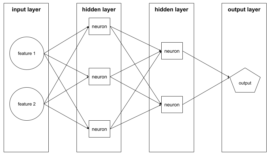
In TensorFlow, layers are also Python functions that take Tensors and configuration options as input and produce other tensors as output.
learning rate
A floating-point number that tells the gradient descent algorithm how strongly to adjust weights and biases on each iteration. For example, a learning rate of 0.3 would adjust weights and biases three times more powerfully than a learning rate of 0.1.
Learning rate is a key hyperparameter. If you set the learning rate too low, training will take too long. If you set the learning rate too high, gradient descent often has trouble reaching convergence.
See Linear regression: Hyperparameters in Machine Learning Crash Course for more information.
linear
A relationship between two or more variables that can be represented solely through addition and multiplication.
The plot of a linear relationship is a line.
Contrast with nonlinear.
linear model
A model that assigns one weight per feature to make predictions. (Linear models also incorporate a bias.) In contrast, the relationship of features to predictions in deep models is generally nonlinear.
Linear models are usually easier to train and more interpretable than deep models. However, deep models can learn complex relationships between features.
Linear regression and logistic regression are two types of linear models.
linear regression
A type of machine learning model in which both of the following are true:
- The model is a linear model.
- The prediction is a floating-point value. (This is the regression part of linear regression.)
Contrast linear regression with logistic regression. Also, contrast regression with classification.
See Linear regression in Machine Learning Crash Course for more information.
logistic regression
A type of regression model that predicts a probability. Logistic regression models have the following characteristics:
- The label is categorical. The term logistic regression usually refers to binary logistic regression, that is, to a model that calculates probabilities for labels with two possible values. A less common variant, multinomial logistic regression, calculates probabilities for labels with more than two possible values.
- The loss function during training is Log Loss. (Multiple Log Loss units can be placed in parallel for labels with more than two possible values.)
- The model has a linear architecture, not a deep neural network. However, the remainder of this definition also applies to deep models that predict probabilities for categorical labels.
For example, consider a logistic regression model that calculates the probability of an input email being either spam or not spam. During inference, suppose the model predicts 0.72. Therefore, the model is estimating:
- A 72% chance of the email being spam.
- A 28% chance of the email not being spam.
A logistic regression model uses the following two-step architecture:
- The model generates a raw prediction (y') by applying a linear function of input features.
- The model uses that raw prediction as input to a sigmoid function, which converts the raw prediction to a value between 0 and 1, exclusive.
Like any regression model, a logistic regression model predicts a number. However, this number typically becomes part of a binary classification model as follows:
- If the predicted number is greater than the classification threshold, the binary classification model predicts the positive class.
- If the predicted number is less than the classification threshold, the binary classification model predicts the negative class.
See Logistic regression in Machine Learning Crash Course for more information.
Log Loss
The loss function used in binary logistic regression.
See Logistic regression: Loss and regularization in Machine Learning Crash Course for more information.
log-odds
The logarithm of the odds of some event.
loss
During the training of a supervised model, a measure of how far a model's prediction is from its label.
A loss function calculates the loss.
See Linear regression: Loss in Machine Learning Crash Course for more information.
loss curve
A plot of loss as a function of the number of training iterations. The following plot shows a typical loss curve:
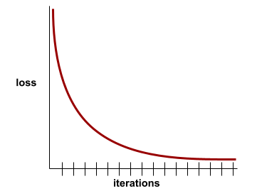
Loss curves can help you determine when your model is converging or overfitting.
Loss curves can plot all of the following types of loss:
See also generalization curve.
See Overfitting: Interpreting loss curves in Machine Learning Crash Course for more information.
loss function
During training or testing, a mathematical function that calculates the loss on a batch of examples. A loss function returns a lower loss for models that makes good predictions than for models that make bad predictions.
The goal of training is typically to minimize the loss that a loss function returns.
Many different kinds of loss functions exist. Pick the appropriate loss function for the kind of model you are building. For example:
- L2 loss (or Mean Squared Error) is the loss function for linear regression.
- Log Loss is the loss function for logistic regression.
M
machine learning
A program or system that trains a model from input data. The trained model can make useful predictions from new (never-before-seen) data drawn from the same distribution as the one used to train the model.
Machine learning also refers to the field of study concerned with these programs or systems.
See the Introduction to Machine Learning course for more information.
majority class
The more common label in a class-imbalanced dataset. For example, given a dataset containing 99% negative labels and 1% positive labels, the negative labels are the majority class.
Contrast with minority class.
See Datasets: Imbalanced datasets in Machine Learning Crash Course for more information.
mini-batch
A small, randomly selected subset of a batch processed in one iteration. The batch size of a mini-batch is usually between 10 and 1,000 examples.
For example, suppose the entire training set (the full batch) consists of 1,000 examples. Further suppose that you set the batch size of each mini-batch to 20. Therefore, each iteration determines the loss on a random 20 of the 1,000 examples and then adjusts the weights and biases accordingly.
It is much more efficient to calculate the loss on a mini-batch than the loss on all the examples in the full batch.
See Linear regression: Hyperparameters in Machine Learning Crash Course for more information.
minority class
The less common label in a class-imbalanced dataset. For example, given a dataset containing 99% negative labels and 1% positive labels, the positive labels are the minority class.
Contrast with majority class.
See Datasets: Imbalanced datasets in Machine Learning Crash Course for more information.
model
In general, any mathematical construct that processes input data and returns output. Phrased differently, a model is the set of parameters and structure needed for a system to make predictions. In supervised machine learning, a model takes an example as input and infers a prediction as output. Within supervised machine learning, models differ somewhat. For example:
- A linear regression model consists of a set of weights and a bias.
- A neural network model consists of:
- A set of hidden layers, each containing one or more neurons.
- The weights and bias associated with each neuron.
- A decision tree model consists of:
- The shape of the tree; that is, the pattern in which the conditions and leaves are connected.
- The conditions and leaves.
You can save, restore, or make copies of a model.
Unsupervised machine learning also generates models, typically a function that can map an input example to the most appropriate cluster.
multi-class classification
In supervised learning, a classification problem in which the dataset contains more than two classes of labels. For example, the labels in the Iris dataset must be one of the following three classes:
- Iris setosa
- Iris virginica
- Iris versicolor
A model trained on the Iris dataset that predicts Iris type on new examples is performing multi-class classification.
In contrast, classification problems that distinguish between exactly two classes are binary classification models. For example, an email model that predicts either spam or not spam is a binary classification model.
In clustering problems, multi-class classification refers to more than two clusters.
See Neural networks: Multi-class classification in Machine Learning Crash Course for more information.
N
negative class
In binary classification, one class is termed positive and the other is termed negative. The positive class is the thing or event that the model is testing for and the negative class is the other possibility. For example:
- The negative class in a medical test might be "not tumor."
- The negative class in an email classification model might be "not spam."
Contrast with positive class.
neural network
A model containing at least one hidden layer. A deep neural network is a type of neural network containing more than one hidden layer. For example, the following diagram shows a deep neural network containing two hidden layers.
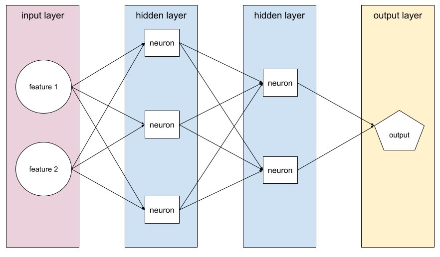
Each neuron in a neural network connects to all of the nodes in the next layer. For example, in the preceding diagram, notice that each of the three neurons in the first hidden layer separately connect to both of the two neurons in the second hidden layer.
Neural networks implemented on computers are sometimes called artificial neural networks to differentiate them from neural networks found in brains and other nervous systems.
Some neural networks can mimic extremely complex nonlinear relationships between different features and the label.
See also convolutional neural network and recurrent neural network.
See Neural networks in Machine Learning Crash Course for more information.
neuron
In machine learning, a distinct unit within a hidden layer of a neural network. Each neuron performs the following two-step action:
- Calculates the weighted sum of input values multiplied by their corresponding weights.
- Passes the weighted sum as input to an activation function.
A neuron in the first hidden layer accepts inputs from the feature values in the input layer. A neuron in any hidden layer beyond the first accepts inputs from the neurons in the preceding hidden layer. For example, a neuron in the second hidden layer accepts inputs from the neurons in the first hidden layer.
The following illustration highlights two neurons and their inputs.
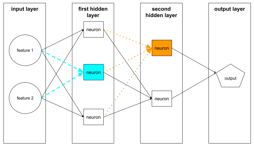
A neuron in a neural network mimics the behavior of neurons in brains and other parts of nervous systems.
node (neural network)
A neuron in a hidden layer.
See Neural Networks in Machine Learning Crash Course for more information.
nonlinear
A relationship between two or more variables that can't be represented solely through addition and multiplication. A linear relationship can be represented as a line; a nonlinear relationship can't be represented as a line. For example, consider two models that each relate a single feature to a single label. The model on the left is linear and the model on the right is nonlinear:
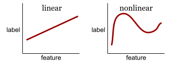
See Neural networks: Nodes and hidden layers in Machine Learning Crash Course to experiment with different kinds of nonlinear functions.
nonstationarity
A feature whose values change across one or more dimensions, usually time. For example, consider the following examples of nonstationarity:
- The number of swimsuits sold at a particular store varies with the season.
- The quantity of a particular fruit harvested in a particular region is zero for much of the year but large for a brief period.
- Due to climate change, annual mean temperatures are shifting.
Contrast with stationarity.
normalization
Broadly speaking, the process of converting a variable's actual range of values into a standard range of values, such as:
- -1 to +1
- 0 to 1
- Z-scores (roughly, -3 to +3)
For example, suppose the actual range of values of a certain feature is 800 to 2,400. As part of feature engineering, you could normalize the actual values down to a standard range, such as -1 to +1.
Normalization is a common task in feature engineering. Models usually train faster (and produce better predictions) when every numerical feature in the feature vector has roughly the same range.
See also Z-score normalization.
See Numerical Data: Normalization in Machine Learning Crash Course for more information.
numerical data
Features represented as integers or real-valued numbers. For example, a house valuation model would probably represent the size of a house (in square feet or square meters) as numerical data. Representing a feature as numerical data indicates that the feature's values have a mathematical relationship to the label. That is, the number of square meters in a house probably has some mathematical relationship to the value of the house.
Not all integer data should be represented as numerical data. For example,
postal codes in some parts of the world are integers; however, integer postal
codes shouldn't be represented as numerical data in models. That's because a
postal code of 20000 is not twice (or half) as potent as a postal code of
10000. Furthermore, although different postal codes do correlate to different
real estate values, we can't assume that real estate values at postal code
20000 are twice as valuable as real estate values at postal code 10000.
Postal codes should be represented as categorical data
instead.
Numerical features are sometimes called continuous features.
See Working with numerical data in Machine Learning Crash Course for more information.
O
offline
Synonym for static.
offline inference
The process of a model generating a batch of predictions and then caching (saving) those predictions. Apps can then access the inferred prediction from the cache rather than rerunning the model.
For example, consider a model that generates local weather forecasts (predictions) once every four hours. After each model run, the system caches all the local weather forecasts. Weather apps retrieve the forecasts from the cache.
Offline inference is also called static inference.
Contrast with online inference. See Production ML systems: Static versus dynamic inference in Machine Learning Crash Course for more information.
one-hot encoding
Representing categorical data as a vector in which:
- One element is set to 1.
- All other elements are set to 0.
One-hot encoding is commonly used to represent strings or identifiers that
have a finite set of possible values.
For example, suppose a certain categorical feature named
Scandinavia has five possible values:
- "Denmark"
- "Sweden"
- "Norway"
- "Finland"
- "Iceland"
One-hot encoding could represent each of the five values as follows:
| Country | Vector | ||||
|---|---|---|---|---|---|
| "Denmark" | 1 | 0 | 0 | 0 | 0 |
| "Sweden" | 0 | 1 | 0 | 0 | 0 |
| "Norway" | 0 | 0 | 1 | 0 | 0 |
| "Finland" | 0 | 0 | 0 | 1 | 0 |
| "Iceland" | 0 | 0 | 0 | 0 | 1 |
Thanks to one-hot encoding, a model can learn different connections based on each of the five countries.
Representing a feature as numerical data is an alternative to one-hot encoding. Unfortunately, representing the Scandinavian countries numerically is not a good choice. For example, consider the following numeric representation:
- "Denmark" is 0
- "Sweden" is 1
- "Norway" is 2
- "Finland" is 3
- "Iceland" is 4
With numeric encoding, a model would interpret the raw numbers mathematically and would try to train on those numbers. However, Iceland isn't actually twice as much (or half as much) of something as Norway, so the model would come to some strange conclusions.
See Categorical data: Vocabulary and one-hot encoding in Machine Learning Crash Course for more information.
one-vs.-all
Given a classification problem with N classes, a solution consisting of N separate binary classification model—one binary classification model for each possible outcome. For example, given a model that classifies examples as animal, vegetable, or mineral, a one-vs.-all solution would provide the following three separate binary classification models:
- animal versus not animal
- vegetable versus not vegetable
- mineral versus not mineral
online
Synonym for dynamic.
online inference
Generating predictions on demand. For example, suppose an app passes input to a model and issues a request for a prediction. A system using online inference responds to the request by running the model (and returning the prediction to the app).
Contrast with offline inference.
See Production ML systems: Static versus dynamic inference in Machine Learning Crash Course for more information.
output layer
The "final" layer of a neural network. The output layer contains the prediction.
The following illustration shows a small deep neural network with an input layer, two hidden layers, and an output layer:
overfitting
Creating a model that matches the training data so closely that the model fails to make correct predictions on new data.
Regularization can reduce overfitting. Training on a large and diverse training set can also reduce overfitting.
See Overfitting in Machine Learning Crash Course for more information.
P
pandas
A column-oriented data analysis API built on top of numpy. Many machine learning frameworks, including TensorFlow, support pandas data structures as inputs. See the pandas documentation for details.
parameter
The weights and biases that a model learns during training. For example, in a linear regression model, the parameters consist of the bias (b) and all the weights (w1, w2, and so on) in the following formula:
In contrast, hyperparameters are the values that you (or a hyperparameter tuning service) supply to the model. For example, learning rate is a hyperparameter.
positive class
The class you are testing for.
For example, the positive class in a cancer model might be "tumor." The positive class in an email classification model might be "spam."
Contrast with negative class.
post-processing
Adjusting the output of a model after the model has been run. Post-processing can be used to enforce fairness constraints without modifying models themselves.
For example, one might apply post-processing to a binary classification model by setting a classification threshold such that equality of opportunity is maintained for some attribute by checking that the true positive rate is the same for all values of that attribute.
precision
A metric for classification models that answers the following question:
When the model predicted the positive class, what percentage of the predictions were correct?
Here is the formula:
where:
- true positive means the model correctly predicted the positive class.
- false positive means the model mistakenly predicted the positive class.
For example, suppose a model made 200 positive predictions. Of these 200 positive predictions:
- 150 were true positives.
- 50 were false positives.
In this case:
Contrast with accuracy and recall.
See Classification: Accuracy, recall, precision and related metrics in Machine Learning Crash Course for more information.
prediction
A model's output. For example:
- The prediction of a binary classification model is either the positive class or the negative class.
- The prediction of a multi-class classification model is one class.
- The prediction of a linear regression model is a number.
proxy labels
Data used to approximate labels not directly available in a dataset.
For example, suppose you must train a model to predict employee stress level. Your dataset contains a lot of predictive features but doesn't contain a label named stress level. Undaunted, you pick "workplace accidents" as a proxy label for stress level. After all, employees under high stress get into more accidents than calm employees. Or do they? Maybe workplace accidents actually rise and fall for multiple reasons.
As a second example, suppose you want is it raining? to be a Boolean label for your dataset, but your dataset doesn't contain rain data. If photographs are available, you might establish pictures of people carrying umbrellas as a proxy label for is it raining? Is that a good proxy label? Possibly, but people in some cultures may be more likely to carry umbrellas to protect against sun than the rain.
Proxy labels are often imperfect. When possible, choose actual labels over proxy labels. That said, when an actual label is absent, pick the proxy label very carefully, choosing the least horrible proxy label candidate.
See Datasets: Labels in Machine Learning Crash Course for more information.
R
RAG
Abbreviation for retrieval-augmented generation.
rater
A human who provides labels for examples. "Annotator" is another name for rater.
See Categorical data: Common issues in Machine Learning Crash Course for more information.
recall
A metric for classification models that answers the following question:
When ground truth was the positive class, what percentage of predictions did the model correctly identify as the positive class?
Here is the formula:
\[\text{Recall} = \frac{\text{true positives}} {\text{true positives} + \text{false negatives}} \]
where:
- true positive means the model correctly predicted the positive class.
- false negative means that the model mistakenly predicted the negative class.
For instance, suppose your model made 200 predictions on examples for which ground truth was the positive class. Of these 200 predictions:
- 180 were true positives.
- 20 were false negatives.
In this case:
\[\text{Recall} = \frac{\text{180}} {\text{180} + \text{20}} = 0.9 \]
See Classification: Accuracy, recall, precision and related metrics for more information.
Rectified Linear Unit (ReLU)
An activation function with the following behavior:
- If input is negative or zero, then the output is 0.
- If input is positive, then the output is equal to the input.
For example:
- If the input is -3, then the output is 0.
- If the input is +3, then the output is 3.0.
Here is a plot of ReLU:
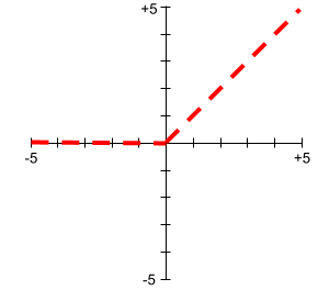
ReLU is a very popular activation function. Despite its simple behavior, ReLU still enables a neural network to learn nonlinear relationships between features and the label.
regression model
Informally, a model that generates a numerical prediction. (In contrast, a classification model generates a class prediction.) For example, the following are all regression models:
- A model that predicts a certain house's value in Euros, such as 423,000.
- A model that predicts a certain tree's life expectancy in years, such as 23.2.
- A model that predicts the amount of rain in inches that will fall in a certain city over the next six hours, such as 0.18.
Two common types of regression models are:
- Linear regression, which finds the line that best fits label values to features.
- Logistic regression, which generates a probability between 0.0 and 1.0 that a system typically then maps to a class prediction.
Not every model that outputs numerical predictions is a regression model. In some cases, a numeric prediction is really just a classification model that happens to have numeric class names. For example, a model that predicts a numeric postal code is a classification model, not a regression model.
regularization
Any mechanism that reduces overfitting. Popular types of regularization include:
- L1 regularization
- L2 regularization
- dropout regularization
- early stopping (this is not a formal regularization method, but can effectively limit overfitting)
Regularization can also be defined as the penalty on a model's complexity.
See Overfitting: Model complexity in Machine Learning Crash Course for more information.
regularization rate
A number that specifies the relative importance of regularization during training. Raising the regularization rate reduces overfitting but may reduce the model's predictive power. Conversely, reducing or omitting the regularization rate increases overfitting.
See Overfitting: L2 regularization in Machine Learning Crash Course for more information.
ReLU
Abbreviation for Rectified Linear Unit.
retrieval-augmented generation (RAG)
A technique for improving the quality of large language model (LLM) output by grounding it with sources of knowledge retrieved after the model was trained. RAG improves the accuracy of LLM responses by providing the trained LLM with access to information retrieved from trusted knowledge bases or documents.
Common motivations to use retrieval-augmented generation include:
- Increasing the factual accuracy of a model's generated responses.
- Giving the model access to knowledge it was not trained on.
- Changing the knowledge that the model uses.
- Enabling the model to cite sources.
For example, suppose that a chemistry app uses the PaLM API to generate summaries related to user queries. When the app's backend receives a query, the backend:
- Searches for ("retrieves") data that's relevant to the user's query.
- Appends ("augments") the relevant chemistry data to the user's query.
- Instructs the LLM to create a summary based on the appended data.
ROC (receiver operating characteristic) Curve
A graph of true positive rate versus false positive rate for different classification thresholds in binary classification.
The shape of an ROC curve suggests a binary classification model's ability to separate positive classes from negative classes. Suppose, for example, that a binary classification model perfectly separates all the negative classes from all the positive classes:

The ROC curve for the preceding model looks as follows:
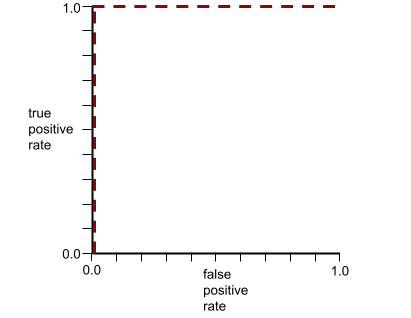
In contrast, the following illustration graphs the raw logistic regression values for a terrible model that can't separate negative classes from positive classes at all:

The ROC curve for this model looks as follows:
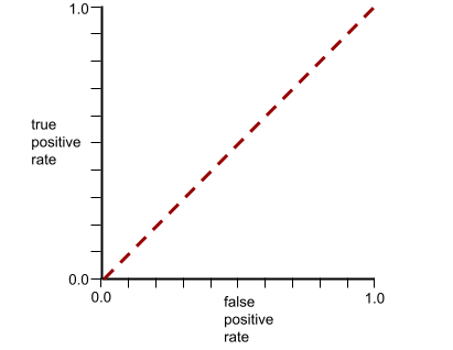
Meanwhile, back in the real world, most binary classification models separate positive and negative classes to some degree, but usually not perfectly. So, a typical ROC curve falls somewhere between the two extremes:
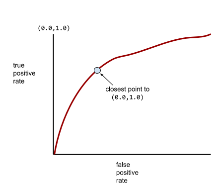
The point on an ROC curve closest to (0.0,1.0) theoretically identifies the ideal classification threshold. However, several other real-world issues influence the selection of the ideal classification threshold. For example, perhaps false negatives cause far more pain than false positives.
A numerical metric called AUC summarizes the ROC curve into a single floating-point value.
Root Mean Squared Error (RMSE)
The square root of the Mean Squared Error.
S
sigmoid function
A mathematical function that "squishes" an input value into a constrained range, typically 0 to 1 or -1 to +1. That is, you can pass any number (two, a million, negative billion, whatever) to a sigmoid and the output will still be in the constrained range. A plot of the sigmoid activation function looks as follows:

The sigmoid function has several uses in machine learning, including:
- Converting the raw output of a logistic regression or multinomial regression model to a probability.
- Acting as an activation function in some neural networks.
softmax
A function that determines probabilities for each possible class in a multi-class classification model. The probabilities add up to exactly 1.0. For example, the following table shows how softmax distributes various probabilities:
| Image is a... | Probability |
|---|---|
| dog | .85 |
| cat | .13 |
| horse | .02 |
Softmax is also called full softmax.
Contrast with candidate sampling.
See Neural networks: Multi-class classification in Machine Learning Crash Course for more information.
sparse feature
A feature whose values are predominately zero or empty. For example, a feature containing a single 1 value and a million 0 values is sparse. In contrast, a dense feature has values that are predominantly not zero or empty.
In machine learning, a surprising number of features are sparse features. Categorical features are usually sparse features. For example, of the 300 possible tree species in a forest, a single example might identify just a maple tree. Or, of the millions of possible videos in a video library, a single example might identify just "Casablanca."
In a model, you typically represent sparse features with one-hot encoding. If the one-hot encoding is big, you might put an embedding layer on top of the one-hot encoding for greater efficiency.
sparse representation
Storing only the position(s) of nonzero elements in a sparse feature.
For example, suppose a categorical feature named species identifies the 36
tree species in a particular forest. Further assume that each
example identifies only a single species.
You could use a one-hot vector to represent the tree species in each example.
A one-hot vector would contain a single 1 (to represent
the particular tree species in that example) and 35 0s (to represent the
35 tree species not in that example). So, the one-hot representation
of maple might look something like the following:

Alternatively, sparse representation would simply identify the position of the
particular species. If maple is at position 24, then the sparse representation
of maple would simply be:
24
Notice that the sparse representation is much more compact than the one-hot representation.
See Working with categorical data in Machine Learning Crash Course for more information.
sparse vector
A vector whose values are mostly zeroes. See also sparse feature and sparsity.
squared loss
Synonym for L2 loss.
static
Something done once rather than continuously. The terms static and offline are synonyms. The following are common uses of static and offline in machine learning:
- static model (or offline model) is a model trained once and then used for a while.
- static training (or offline training) is the process of training a static model.
- static inference (or offline inference) is a process in which a model generates a batch of predictions at a time.
Contrast with dynamic.
static inference
Synonym for offline inference.
stationarity
A feature whose values don't change across one or more dimensions, usually time. For example, a feature whose values look about the same in 2021 and 2023 exhibits stationarity.
In the real world, very few features exhibit stationarity. Even features synonymous with stability (like sea level) change over time.
Contrast with nonstationarity.
stochastic gradient descent (SGD)
A gradient descent algorithm in which the batch size is one. In other words, SGD trains on a single example chosen uniformly at random from a training set.
See Linear regression: Hyperparameters in Machine Learning Crash Course for more information.
supervised machine learning
Training a model from features and their corresponding labels. Supervised machine learning is analogous to learning a subject by studying a set of questions and their corresponding answers. After mastering the mapping between questions and answers, a student can then provide answers to new (never-before-seen) questions on the same topic.
Compare with unsupervised machine learning.
See Supervised Learning in the Introduction to ML course for more information.
synthetic feature
A feature not present among the input features, but assembled from one or more of them. Methods for creating synthetic features include the following:
- Bucketing a continuous feature into range bins.
- Creating a feature cross.
- Multiplying (or dividing) one feature value by other feature value(s)
or by itself. For example, if
aandbare input features, then the following are examples of synthetic features:- ab
- a2
- Applying a transcendental function to a feature value. For example, if
cis an input feature, then the following are examples of synthetic features:- sin(c)
- ln(c)
Features created by normalizing or scaling alone are not considered synthetic features.
T
test loss
A metric representing a model's loss against the test set. When building a model, you typically try to minimize test loss. That's because a low test loss is a stronger quality signal than a low training loss or low validation loss.
A large gap between test loss and training loss or validation loss sometimes suggests that you need to increase the regularization rate.
training
The process of determining the ideal parameters (weights and biases) comprising a model. During training, a system reads in examples and gradually adjusts parameters. Training uses each example anywhere from a few times to billions of times.
See Supervised Learning in the Introduction to ML course for more information.
training loss
A metric representing a model's loss during a particular training iteration. For example, suppose the loss function is Mean Squared Error. Perhaps the training loss (the Mean Squared Error) for the 10th iteration is 2.2, and the training loss for the 100th iteration is 1.9.
A loss curve plots training loss versus the number of iterations. A loss curve provides the following hints about training:
- A downward slope implies that the model is improving.
- An upward slope implies that the model is getting worse.
- A flat slope implies that the model has reached convergence.
For example, the following somewhat idealized loss curve shows:
- A steep downward slope during the initial iterations, which implies rapid model improvement.
- A gradually flattening (but still downward) slope until close to the end of training, which implies continued model improvement at a somewhat slower pace then during the initial iterations.
- A flat slope towards the end of training, which suggests convergence.

Although training loss is important, see also generalization.
training-serving skew
The difference between a model's performance during training and that same model's performance during serving.
training set
The subset of the dataset used to train a model.
Traditionally, examples in the dataset are divided into the following three distinct subsets:
- a training set
- a validation set
- a test set
Ideally, each example in the dataset should belong to only one of the preceding subsets. For example, a single example shouldn't belong to both the training set and the validation set.
See Datasets: Dividing the original dataset in Machine Learning Crash Course for more information.
true negative (TN)
An example in which the model correctly predicts the negative class. For example, the model infers that a particular email message is not spam, and that email message really is not spam.
true positive (TP)
An example in which the model correctly predicts the positive class. For example, the model infers that a particular email message is spam, and that email message really is spam.
true positive rate (TPR)
Synonym for recall. That is:
True positive rate is the y-axis in an ROC curve.
U
underfitting
Producing a model with poor predictive ability because the model hasn't fully captured the complexity of the training data. Many problems can cause underfitting, including:
- Training on the wrong set of features.
- Training for too few epochs or at too low a learning rate.
- Training with too high a regularization rate.
- Providing too few hidden layers in a deep neural network.
See Overfitting in Machine Learning Crash Course for more information.
unlabeled example
An example that contains features but no label. For example, the following table shows three unlabeled examples from a house valuation model, each with three features but no house value:
| Number of bedrooms | Number of bathrooms | House age |
|---|---|---|
| 3 | 2 | 15 |
| 2 | 1 | 72 |
| 4 | 2 | 34 |
In supervised machine learning, models train on labeled examples and make predictions on unlabeled examples.
In semi-supervised and unsupervised learning, unlabeled examples are used during training.
Contrast unlabeled example with labeled example.
unsupervised machine learning
Training a model to find patterns in a dataset, typically an unlabeled dataset.
The most common use of unsupervised machine learning is to cluster data into groups of similar examples. For example, an unsupervised machine learning algorithm can cluster songs based on various properties of the music. The resulting clusters can become an input to other machine learning algorithms (for example, to a music recommendation service). Clustering can help when useful labels are scarce or absent. For example, in domains such as anti-abuse and fraud, clusters can help humans better understand the data.
Contrast with supervised machine learning.
See What is Machine Learning? in the Introduction to ML course for more information.
V
validation
The initial evaluation of a model's quality. Validation checks the quality of a model's predictions against the validation set.
Because the validation set differs from the training set, validation helps guard against overfitting.
You might think of evaluating the model against the validation set as the first round of testing and evaluating the model against the test set as the second round of testing.
validation loss
A metric representing a model's loss on the validation set during a particular iteration of training.
See also generalization curve.
validation set
The subset of the dataset that performs initial evaluation against a trained model. Typically, you evaluate the trained model against the validation set several times before evaluating the model against the test set.
Traditionally, you divide the examples in the dataset into the following three distinct subsets:
- a training set
- a validation set
- a test set
Ideally, each example in the dataset should belong to only one of the preceding subsets. For example, a single example shouldn't belong to both the training set and the validation set.
See Datasets: Dividing the original dataset in Machine Learning Crash Course for more information.
W
weight
A value that a model multiplies by another value. Training is the process of determining a model's ideal weights; inference is the process of using those learned weights to make predictions.
See Linear regression in Machine Learning Crash Course for more information.
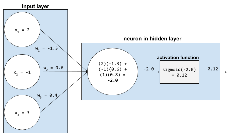
weighted sum
The sum of all the relevant input values multiplied by their corresponding weights. For example, suppose the relevant inputs consist of the following:
| input value | input weight |
| 2 | -1.3 |
| -1 | 0.6 |
| 3 | 0.4 |
The weighted sum is therefore:
weighted sum = (2)(-1.3) + (-1)(0.6) + (3)(0.4) = -2.0
A weighted sum is the input argument to an activation function.
Z
Z-score normalization
A scaling technique that replaces a raw feature value with a floating-point value representing the number of standard deviations from that feature's mean. For example, consider a feature whose mean is 800 and whose standard deviation is 100. The following table shows how Z-score normalization would map the raw value to its Z-score:
| Raw value | Z-score |
|---|---|
| 800 | 0 |
| 950 | +1.5 |
| 575 | -2.25 |
The machine learning model then trains on the Z-scores for that feature instead of on the raw values.
See Numerical data: Normalization in Machine Learning Crash Course for more information.
