این صفحه شامل اصطلاحات واژهنامه اصول یادگیری ماشین است. برای مشاهده همه اصطلاحات واژهنامه، اینجا کلیک کنید .
الف
دقت
تعداد پیشبینیهای طبقهبندی صحیح تقسیم بر تعداد کل پیشبینیها. یعنی:
برای مثال، مدلی که ۴۰ پیشبینی درست و ۱۰ پیشبینی نادرست انجام داده باشد، دقتی برابر با:
طبقهبندی دودویی نامهای خاصی را برای دستههای مختلف پیشبینیهای درست و پیشبینیهای نادرست ارائه میدهد. بنابراین، فرمول دقت برای طبقهبندی دودویی به شرح زیر است:
کجا:
- TP تعداد موارد مثبت واقعی (پیشبینیهای صحیح) است.
- TN تعداد منفیهای واقعی (پیشبینیهای صحیح) است.
- FP تعداد مثبتهای کاذب (پیشبینیهای نادرست) است.
- FN تعداد نتایج منفی کاذب (پیشبینیهای نادرست) است.
دقت را با دقت و یادآوری مقایسه و مقابله کنید.
برای اطلاعات بیشتر به بخش طبقهبندی: دقت، فراخوانی، دقت و معیارهای مرتبط در دوره فشرده یادگیری ماشین مراجعه کنید.
تابع فعالسازی
تابعی که شبکههای عصبی را قادر میسازد روابط غیرخطی (پیچیده) بین ویژگیها و برچسب را یاد بگیرند.
توابع فعالسازی محبوب عبارتند از:
نمودارهای توابع فعالسازی هرگز به صورت خطوط مستقیم منفرد نیستند. برای مثال، نمودار تابع فعالسازی ReLU از دو خط مستقیم تشکیل شده است:

نمودار تابع فعالسازی سیگموئید به شکل زیر است:

برای دیدن مثال روی آیکون کلیک کنید.
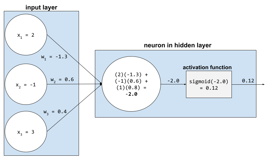
در یک شبکه عصبی، توابع فعالسازی، مجموع وزنی تمام ورودیهای یک نورون را دستکاری میکنند. برای محاسبه مجموع وزنی، نورون حاصلضرب مقادیر و وزنهای مربوطه را جمع میکند. برای مثال، فرض کنید ورودی مربوطه به یک نورون شامل موارد زیر باشد:
| مقدار ورودی | وزن ورودی |
| ۲ | -۱.۳ |
| -1 | ۰.۶ |
| ۳ | ۰.۴ |
weighted sum = (2)(-1.3) + (-1)(0.6) + (3)(0.4) = -2.0
برای اطلاعات بیشتر به بخش شبکههای عصبی: توابع فعالسازی در دوره فشرده یادگیری ماشین مراجعه کنید.
هوش مصنوعی
یک برنامه یا مدل غیرانسانی که میتواند وظایف پیچیده را حل کند. به عنوان مثال، برنامه یا مدلی که متن را ترجمه میکند یا برنامه یا مدلی که بیماریها را از تصاویر رادیولوژی شناسایی میکند، هر دو هوش مصنوعی را نشان میدهند.
بهطور رسمی، یادگیری ماشینی زیرمجموعهای از هوش مصنوعی است. با این حال، در سالهای اخیر، برخی سازمانها شروع به استفاده از اصطلاحات هوش مصنوعی و یادگیری ماشینی به جای یکدیگر کردهاند.
AUC (مساحت زیر منحنی ROC)
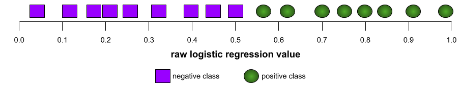
عددی بین ۰.۰ و ۱.۰ که نشاندهنده توانایی یک مدل طبقهبندی دودویی در جداسازی کلاسهای مثبت از کلاسهای منفی است. هرچه AUC به ۱.۰ نزدیکتر باشد، توانایی مدل در جداسازی کلاسها از یکدیگر بهتر است.
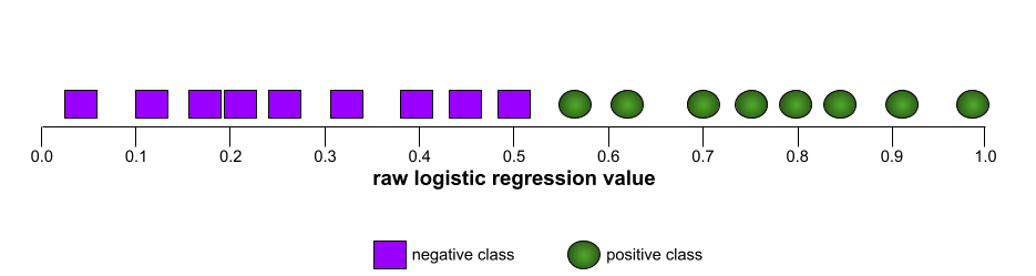
برای مثال، تصویر زیر یک مدل طبقهبندی را نشان میدهد که کلاسهای مثبت (بیضیهای سبز) را از کلاسهای منفی (مستطیلهای بنفش) به طور کامل جدا میکند. این مدل که به طور غیرواقعی بینقص است، AUC برابر با ۱.۰ دارد:
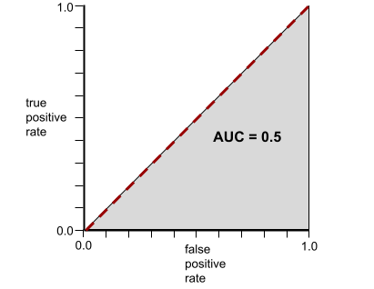
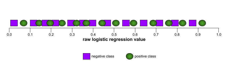
برعکس، تصویر زیر نتایج یک مدل طبقهبندی را نشان میدهد که نتایج تصادفی تولید کرده است. این مدل دارای AUC برابر با 0.5 است:
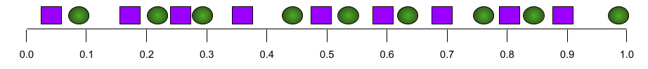
بله، مدل قبلی AUC برابر با 0.5 دارد، نه 0.0.
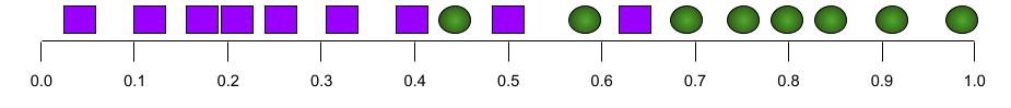
بیشتر مدلها جایی بین این دو حالت افراطی قرار دارند. برای مثال، مدل زیر تا حدودی موارد مثبت را از موارد منفی جدا میکند و بنابراین AUC آن بین 0.5 تا 1.0 است:
AUC هر مقداری را که برای آستانه طبقهبندی تعیین میکنید، نادیده میگیرد. در عوض، AUC تمام آستانههای طبقهبندی ممکن را در نظر میگیرد.
برای آشنایی با رابطه بین منحنیهای AUC و ROC، روی آیکون کلیک کنید.
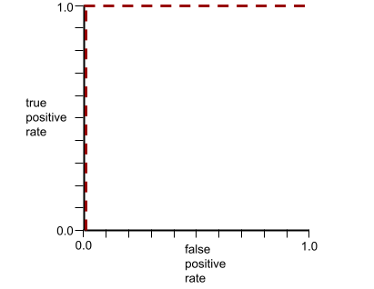
AUC نشان دهنده مساحت زیر منحنی ROC است. برای مثال، منحنی ROC برای مدلی که به طور کامل موارد مثبت را از موارد منفی جدا میکند، به شکل زیر است:
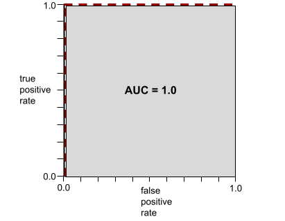
AUC مساحت ناحیه خاکستری در تصویر قبلی است. در این مورد غیرمعمول، مساحت به سادگی حاصل ضرب طول ناحیه خاکستری (1.0) در عرض ناحیه خاکستری (1.0) است. بنابراین، حاصل ضرب 1.0 و 1.0، AUC دقیقاً 1.0 را به دست میدهد که بالاترین امتیاز AUC ممکن است.
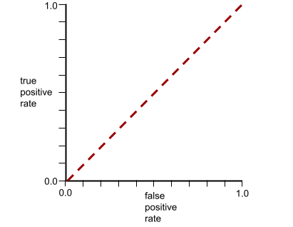
برعکس، منحنی ROC برای یک مدل طبقهبندی که اصلاً نمیتواند کلاسها را از هم جدا کند به صورت زیر است. مساحت این ناحیه خاکستری 0.5 است.
یک منحنی ROC معمولیتر تقریباً شبیه به شکل زیر است:
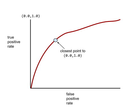
محاسبهی دستی مساحت زیر این منحنی کار دشواری خواهد بود، به همین دلیل است که معمولاً یک برنامه بیشتر مقادیر AUC را محاسبه میکند.
برای اطلاعات بیشتر به بخش طبقهبندی: ROC و AUC در دوره فشرده یادگیری ماشین مراجعه کنید.
ب
پسانتشار
الگوریتمی که گرادیان نزولی را در شبکههای عصبی پیادهسازی میکند.
آموزش یک شبکه عصبی شامل تکرارهای زیادی از چرخه دو مرحلهای زیر است:
- در طول مرحلهی رو به جلو ، سیستم مجموعهای از مثالها را برای ارائه پیشبینی(ها) پردازش میکند. سیستم هر پیشبینی را با هر مقدار برچسب مقایسه میکند. تفاوت بین پیشبینی و مقدار برچسب، میزان زیان آن مثال است. سیستم زیانهای مربوط به تمام مثالها را جمع میکند تا کل زیان برای دسته فعلی را محاسبه کند.
- در طول فرآیند پسانتشار (backpropagation)، سیستم با تنظیم وزن تمام نورونها در تمام لایههای پنهان، تلفات را کاهش میدهد.
شبکههای عصبی اغلب شامل نورونهای زیادی در لایههای پنهان متعدد هستند. هر یک از این نورونها به روشهای مختلفی در کاهش کلی نقش دارند. پسانتشار تعیین میکند که آیا وزنهای اعمال شده به نورونهای خاص افزایش یا کاهش یابد.
نرخ یادگیری ضریبی است که میزان افزایش یا کاهش هر وزن را در هر بار عبور از الگوریتم به عقب کنترل میکند. نرخ یادگیری بزرگ، هر وزن را بیشتر از نرخ یادگیری کوچک افزایش یا کاهش میدهد.
به زبان حسابان، پسانتشار، قاعده زنجیرهای را از حسابان پیادهسازی میکند. یعنی، پسانتشار، مشتق جزئی خطا را نسبت به هر پارامتر محاسبه میکند.
سالها پیش، متخصصان یادگیری ماشین مجبور بودند برای پیادهسازی پسانتشار کد بنویسند. رابطهای برنامهنویسی کاربردی (API) مدرن یادگیری ماشین مانند Keras اکنون پسانتشار را برای شما پیادهسازی میکنند. وای!
برای اطلاعات بیشتر به بخش شبکههای عصبی در دوره فشرده یادگیری ماشین مراجعه کنید.
دستهای
مجموعه مثالهای استفاده شده در یک تکرار آموزشی. اندازه دسته، تعداد مثالها در یک دسته را تعیین میکند.
برای توضیح چگونگی ارتباط یک دسته با یک دوره، به epoch مراجعه کنید.
برای اطلاعات بیشتر به رگرسیون خطی: هایپرپارامترها در دوره فشرده یادگیری ماشین مراجعه کنید.
اندازه دسته
تعداد مثالها در یک دسته . برای مثال، اگر اندازه دسته ۱۰۰ باشد، مدل در هر تکرار ۱۰۰ مثال را پردازش میکند.
موارد زیر استراتژیهای رایج برای اندازه دستهای هستند:
- نزول گرادیان تصادفی (SGD) ، که در آن اندازه دسته ۱ است.
- دسته کامل، که در آن اندازه دسته برابر با تعداد مثالها در کل مجموعه آموزشی است. برای مثال، اگر مجموعه آموزشی شامل یک میلیون مثال باشد، اندازه دسته نیز یک میلیون مثال خواهد بود. دسته کامل معمولاً یک استراتژی ناکارآمد است.
- مینی-بچ که در آن اندازه هر دسته معمولاً بین ۱۰ تا ۱۰۰۰ است. مینی-بچ معمولاً کارآمدترین استراتژی است.
برای اطلاعات بیشتر به موارد زیر مراجعه کنید:
- سیستمهای یادگیری ماشینی تولیدی: استنتاج ایستا در مقابل استنتاج پویا در دوره فشرده یادگیری ماشین.
- کتابچه راهنمای تنظیم یادگیری عمیق .
جانبداری (اخلاق/انصاف)
۱. کلیشهسازی، تعصب یا جانبداری نسبت به برخی چیزها، افراد یا گروهها نسبت به برخی دیگر. این سوگیریها میتوانند بر جمعآوری و تفسیر دادهها، طراحی سیستم و نحوه تعامل کاربران با سیستم تأثیر بگذارند. انواع این نوع سوگیری عبارتند از:
- سوگیری اتوماسیون
- سوگیری تأییدی
- سوگیری آزمایشگر
- سوگیری انتساب گروهی
- سوگیری ضمنی
- سوگیری درون گروهی
- سوگیری همگنی برونگروهی
۲. خطای سیستماتیک ناشی از یک روش نمونهگیری یا گزارشدهی. انواع این نوع سوگیری عبارتند از:
نباید با اصطلاح سوگیری در مدلهای یادگیری ماشین یا سوگیری پیشبینی اشتباه گرفته شود.
برای اطلاعات بیشتر به انصاف: انواع سوگیری در دوره فشرده یادگیری ماشین مراجعه کنید.
بایاس (ریاضی) یا اصطلاح بایاس
یک تقاطع یا انحراف از یک مبدا. بایاس (Bias) یک پارامتر در مدلهای یادگیری ماشین است که با یکی از موارد زیر نمایش داده میشود:
- ب
- w 0
برای مثال، بایاس در فرمول زیر برابر با b است:
در یک خط ساده دو بعدی، بایاس فقط به معنای "عرض از مبدا" است. برای مثال، بایاس خط در تصویر زیر ۲ است.
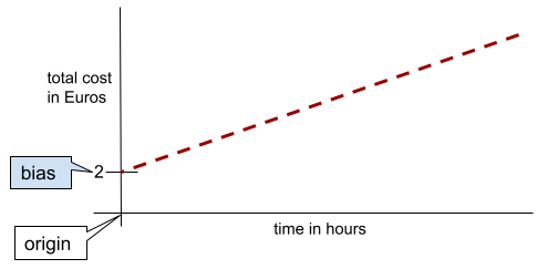
سوگیری وجود دارد زیرا همه مدلها از مبدا (0,0) شروع نمیشوند. برای مثال، فرض کنید هزینه ورود به یک شهربازی 2 یورو و به ازای هر ساعت اقامت مشتری 0.5 یورو اضافی است. بنابراین، مدلی که هزینه کل را ترسیم میکند، سوگیری 2 دارد زیرا کمترین هزینه 2 یورو است.
سوگیری را نباید با سوگیری در اخلاق و انصاف یا سوگیری در پیشبینی اشتباه گرفت.
برای اطلاعات بیشتر به دوره فشرده رگرسیون خطی در یادگیری ماشین مراجعه کنید.
طبقهبندی دودویی
نوعی وظیفه طبقهبندی که یکی از دو کلاس ناسازگار را پیشبینی میکند:
برای مثال، دو مدل یادگیری ماشین زیر هر کدام طبقهبندی دودویی را انجام میدهند:
- مدلی که تعیین میکند آیا پیامهای ایمیل هرزنامه (دسته مثبت) هستند یا هرزنامه (دسته منفی).
- مدلی که علائم پزشکی را ارزیابی میکند تا مشخص کند که آیا فرد بیماری خاصی دارد (دسته مثبت) یا آن بیماری را ندارد (دسته منفی).
مقایسه با طبقهبندی چند طبقهای
همچنین به رگرسیون لجستیک و آستانه طبقهبندی مراجعه کنید.
برای اطلاعات بیشتر به بخش طبقهبندی در دوره فشرده یادگیری ماشین مراجعه کنید.
سطل زدن
تبدیل یک ویژگی واحد به چندین ویژگی دودویی به نام سطل یا سطل ، که معمولاً بر اساس یک محدوده مقدار انجام میشود. ویژگی خرد شده معمولاً یک ویژگی پیوسته است.
برای مثال، به جای نمایش دما به عنوان یک ویژگی ممیز شناور پیوسته، میتوانید محدودههای دما را به بخشهای گسسته تقسیم کنید، مانند:
- کمتر یا مساوی ۱۰ درجه سانتیگراد، سطل «سرد» خواهد بود.
- دمای ۱۱ تا ۲۴ درجه سانتیگراد، دمای «معتدل» خواهد بود.
- دمای بالاتر از ۲۵ درجه سانتیگراد، سطل «گرم» خواهد بود.
این مدل با هر مقدار در یک سطل به طور یکسان رفتار خواهد کرد. برای مثال، مقادیر 13 و 22 هر دو در سطل معتدل هستند، بنابراین مدل با این دو مقدار به طور یکسان رفتار میکند.
برای اطلاعات بیشتر به دوره فشرده دادههای عددی: ادغام در یادگیری ماشین مراجعه کنید.
سی
دادههای دستهبندیشده
ویژگیهایی که مجموعهای خاص از مقادیر ممکن را دارند. برای مثال، یک ویژگی دستهبندیشده به نام traffic-light-state را در نظر بگیرید که فقط میتواند یکی از سه مقدار ممکن زیر را داشته باشد:
-
red -
yellow -
green
با نمایش traffic-light-state به عنوان یک ویژگی دستهبندیشده، یک مدل میتواند تأثیرات متفاوت رنگهای red ، green و yellow را بر رفتار راننده بیاموزد.
ویژگیهای دستهبندیشده گاهی اوقات ویژگیهای گسسته نامیده میشوند.
با دادههای عددی مقایسه کنید.
برای اطلاعات بیشتر به بخش «کار با دادههای دستهبندیشده» در دوره فشرده یادگیری ماشین مراجعه کنید.
کلاس
دستهای که یک برچسب میتواند به آن تعلق داشته باشد. برای مثال:
- در یک مدل طبقهبندی دودویی که هرزنامه را تشخیص میدهد، دو کلاس ممکن است هرزنامه باشند و هرزنامه نباشند .
- در یک مدل طبقهبندی چندکلاسه که نژادهای سگ را شناسایی میکند، کلاسها ممکن است پودل ، بیگل ، پاگ و غیره باشند.
یک مدل طبقهبندی، یک کلاس را پیشبینی میکند. در مقابل، یک مدل رگرسیون به جای یک کلاس، یک عدد را پیشبینی میکند.
برای اطلاعات بیشتر به بخش طبقهبندی در دوره فشرده یادگیری ماشین مراجعه کنید.
مدل طبقهبندی
مدلی که پیشبینی آن یک کلاس است. برای مثال، مدلهای زیر همگی مدلهای طبقهبندی هستند:
- مدلی که زبان جمله ورودی (فرانسوی؟ اسپانیایی؟ ایتالیایی؟) را پیشبینی میکند.
- مدلی که گونههای درختی (افرا؟ بلوط؟ بائوباب؟) را پیشبینی میکند.
- مدلی که کلاس مثبت یا منفی را برای یک وضعیت پزشکی خاص پیشبینی میکند.
در مقابل، مدلهای رگرسیون به جای کلاسها، اعداد را پیشبینی میکنند.
دو نوع رایج از مدلهای طبقهبندی عبارتند از:
آستانه طبقهبندی
در یک طبقهبندی دودویی ، عددی بین ۰ و ۱ که خروجی خام یک مدل رگرسیون لجستیک را به پیشبینی کلاس مثبت یا کلاس منفی تبدیل میکند. توجه داشته باشید که آستانه طبقهبندی مقداری است که انسان انتخاب میکند، نه مقداری که توسط آموزش مدل انتخاب شده است.
یک مدل رگرسیون لجستیک یک مقدار خام بین ۰ و ۱ را خروجی میدهد. سپس:
- اگر این مقدار خام بزرگتر از آستانه طبقهبندی باشد، آنگاه کلاس مثبت پیشبینی میشود.
- اگر این مقدار خام کمتر از آستانه طبقهبندی باشد، آنگاه کلاس منفی پیشبینی میشود.
برای مثال، فرض کنید آستانه طبقهبندی ۰.۸ باشد. اگر مقدار خام ۰.۹ باشد، مدل کلاس مثبت را پیشبینی میکند. اگر مقدار خام ۰.۷ باشد، مدل کلاس منفی را پیشبینی میکند.
انتخاب آستانه طبقهبندی به شدت بر تعداد موارد مثبت کاذب و منفی کاذب تأثیر میگذارد.
برای اطلاعات بیشتر به بخش آستانهها و ماتریس درهمریختگی در دوره فشرده یادگیری ماشین مراجعه کنید.
طبقه بندی کننده
یک اصطلاح غیررسمی برای یک مدل طبقهبندی .
مجموعه داده نامتوازن از نظر کلاس
یک مجموعه داده برای طبقهبندی که در آن تعداد کل برچسبهای هر کلاس به طور قابل توجهی متفاوت است. به عنوان مثال، یک مجموعه داده طبقهبندی دودویی را در نظر بگیرید که دو برچسب آن به صورت زیر تقسیم شدهاند:
- ۱،۰۰۰،۰۰۰ برچسب منفی
- ۱۰ برچسب مثبت
نسبت برچسبهای منفی به مثبت ۱۰۰۰۰۰ به ۱ است، بنابراین این یک مجموعه داده نامتعادل از نظر کلاس است.
در مقابل، مجموعه داده زیر از نظر کلاس متعادل است زیرا نسبت برچسبهای منفی به برچسبهای مثبت نسبتاً نزدیک به ۱ است:
- ۵۱۷ برچسب منفی
- ۴۸۳ برچسب مثبت
مجموعه دادههای چند کلاسه همچنین میتوانند از نظر کلاس نامتعادل باشند. برای مثال، مجموعه دادههای طبقهبندی چند کلاسه زیر نیز از نظر کلاس نامتعادل است زیرا یک برچسب نمونههای بسیار بیشتری نسبت به دو برچسب دیگر دارد:
- ۱,۰۰۰,۰۰۰ برچسب با کلاس «سبز»
- ۲۰۰ برچسب با کلاس «بنفش»
- ۳۵۰ برچسب با کلاس «نارنجی»
آموزش مجموعه دادههای نامتوازن از نظر کلاس میتواند چالشهای خاصی را ایجاد کند. برای جزئیات بیشتر به بخش مجموعه دادههای نامتوازن در دوره فشرده یادگیری ماشین مراجعه کنید.
همچنین به آنتروپی ، کلاس اکثریت و کلاس اقلیت مراجعه کنید.
برش
تکنیکی برای مدیریت دادههای پرت با انجام یک یا هر دو مورد زیر:
- کاهش مقادیر ویژگیهایی که از یک آستانه حداکثر بزرگتر هستند تا رسیدن به آن آستانه حداکثر.
- افزایش مقادیر ویژگیهایی که کمتر از یک آستانه حداقل هستند تا آن آستانه حداقل.
برای مثال، فرض کنید که کمتر از ۰.۵٪ از مقادیر برای یک ویژگی خاص خارج از محدوده ۴۰ تا ۶۰ قرار میگیرند. در این حالت، میتوانید موارد زیر را انجام دهید:
- تمام مقادیر بالای ۶۰ (حداکثر آستانه) را طوری برش دهید که دقیقاً ۶۰ باشند.
- تمام مقادیر زیر ۴۰ (حداقل آستانه) را طوری برش دهید که دقیقاً ۴۰ باشند.
دادههای پرت میتوانند به مدلها آسیب بزنند، و گاهی اوقات باعث سرریز وزنها در طول آموزش میشوند. برخی از دادههای پرت همچنین میتوانند معیارهایی مانند دقت را به طور چشمگیری خراب کنند. حذف دادهها یک تکنیک رایج برای محدود کردن آسیب است.
برش گرادیان ، مقادیر گرادیان را در طول آموزش در محدوده تعیینشدهای قرار میدهد.
برای اطلاعات بیشتر به دوره فشرده دادههای عددی: نرمالسازی در یادگیری ماشین مراجعه کنید.
ماتریس سردرگمی
یک جدول NxN که تعداد پیشبینیهای صحیح و نادرست انجام شده توسط یک مدل طبقهبندی را خلاصه میکند. برای مثال، ماتریس درهمریختگی زیر را برای یک مدل طبقهبندی دودویی در نظر بگیرید:
| تومور (پیشبینیشده) | غیر توموری (پیشبینیشده) | |
|---|---|---|
| تومور (حقیقت زمینی) | ۱۸ (تی پی) | ۱ (FN) |
| غیر توموری (حقیقت زمینی) | ۶ (FP) | ۴۵۲ (تنسی) |
ماتریس درهمریختگی قبلی موارد زیر را نشان میدهد:
- از ۱۹ پیشبینی که در آنها حقیقت زمینهای تومور بود، مدل ۱۸ مورد را به درستی طبقهبندی کرد و ۱ مورد را به اشتباه طبقهبندی کرد.
- از ۴۵۸ پیشبینی که در آنها حقیقت زمینهای غیرتومور بود، مدل ۴۵۲ مورد را به درستی طبقهبندی کرد و ۶ مورد را به اشتباه طبقهبندی کرد.
ماتریس سردرگمی برای یک مسئله طبقهبندی چند کلاسه میتواند به شما در شناسایی الگوهای اشتباه کمک کند. برای مثال، ماتریس سردرگمی زیر را برای یک مدل طبقهبندی چند کلاسه ۳ کلاسه در نظر بگیرید که سه نوع عنبیه مختلف (ویرجینیکا، ورسیکالر و ستوسا) را دستهبندی میکند. وقتی حقیقت زمینهای ویرجینیکا بود، ماتریس سردرگمی نشان میدهد که احتمال پیشبینی اشتباه ورسیکالر توسط مدل بسیار بیشتر از ستوسا بوده است:
| ستوسا (پیشبینیشده) | ورسیکالر (پیشبینیشده) | ویرجینیکا (پیشبینیشده) | |
|---|---|---|---|
| ستوسا (حقیقت زمینی) | ۸۸ | ۱۲ | 0 |
| ورسیکالر (حقیقت زمینی) | ۶ | ۱۴۱ | ۷ |
| ویرجینیکا (حقیقت زمینی) | ۲ | ۲۷ | ۱۰۹ |
به عنوان مثالی دیگر، یک ماتریس درهمریختگی میتواند نشان دهد که مدلی که برای تشخیص ارقام دستنویس آموزش دیده است، تمایل دارد به اشتباه عدد ۹ را به جای ۴ یا به اشتباه عدد ۱ را به جای ۷ پیشبینی کند.
ماتریسهای درهمریختگی حاوی اطلاعات کافی برای محاسبهی انواع معیارهای عملکرد، از جمله دقت و فراخوانی، هستند.
ویژگی پیوسته
یک ویژگی ممیز شناور با طیف نامحدودی از مقادیر ممکن، مانند دما یا وزن.
تضاد با ویژگی گسسته .
همگرایی
حالتی که در آن مقادیر تلفات با هر تکرار بسیار کم یا اصلاً تغییر نمیکنند. برای مثال، منحنی تلفات زیر همگرایی را در حدود ۷۰۰ تکرار نشان میدهد:
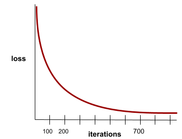
یک مدل زمانی همگرا میشود که آموزش اضافی، مدل را بهبود نبخشد.
در یادگیری عمیق ، مقادیر زیان گاهی اوقات برای بسیاری از تکرارها ثابت یا تقریباً ثابت میمانند تا اینکه در نهایت کاهش مییابند. در طول یک دوره طولانی از مقادیر زیان ثابت، ممکن است به طور موقت حس کاذبی از همگرایی داشته باشید.
همچنین به توقف زودهنگام مراجعه کنید.
برای اطلاعات بیشتر به منحنیهای همگرایی و تلفات مدل در دوره فشرده یادگیری ماشین مراجعه کنید.
دی
قاب داده
یک نوع داده محبوب پانداس برای نمایش مجموعه دادهها در حافظه.
یک DataFrame مشابه یک جدول یا صفحه گسترده است. هر ستون از DataFrame یک نام (سربرگ) دارد و هر سطر با یک شماره منحصر به فرد مشخص میشود.
هر ستون در یک DataFrame مانند یک آرایه دوبعدی ساختار یافته است، با این تفاوت که به هر ستون میتوان نوع داده خاص خود را اختصاص داد.
همچنین به صفحه مرجع رسمی pandas.DataFrame مراجعه کنید.
مجموعه داده یا دیتاست
مجموعهای از دادههای خام، که معمولاً (اما نه منحصراً) در یکی از قالبهای زیر سازماندهی میشوند:
- یک صفحه گسترده
- فایلی با فرمت CSV (مقادیر جدا شده با کاما)
مدل عمیق
یک شبکه عصبی شامل بیش از یک لایه پنهان .
یک مدل عمیق، شبکه عصبی عمیق نیز نامیده میشود.
با مدل عریض در تضاد باشید.
ویژگی متراکم
ویژگیای که در آن بیشتر یا همه مقادیر غیرصفر هستند، معمولاً یک تانسور از مقادیر اعشاری. برای مثال، تانسور 10 عنصری زیر متراکم است زیرا 9 مقدار از مقادیر آن غیرصفر هستند:
| ۸ | ۳ | ۷ | ۵ | ۲ | ۴ | 0 | ۴ | ۹ | ۶ |
تضاد با ویژگی پراکنده .
عمق
مجموع موارد زیر در یک شبکه عصبی :
- تعداد لایههای پنهان
- تعداد لایههای خروجی ، که معمولاً ۱ است
- تعداد هر لایه جاسازی شده
برای مثال، یک شبکه عصبی با پنج لایه پنهان و یک لایه خروجی، عمق ۶ دارد.
توجه داشته باشید که لایه ورودی تاثیری بر عمق ندارد.
ویژگی گسسته
یک ویژگی با مجموعهای متناهی از مقادیر ممکن. برای مثال، ویژگیای که مقادیر آن فقط میتواند حیوانی ، گیاهی یا معدنی باشد، یک ویژگی گسسته (یا دستهبندیشده) است.
کنتراست با ویژگی پیوسته .
پویا
کاری که به طور مکرر یا مداوم انجام میشود. اصطلاحات پویا و آنلاین در یادگیری ماشین مترادف هستند. موارد زیر کاربردهای رایج پویا و آنلاین در یادگیری ماشین است:
- یک مدل پویا (یا مدل آنلاین ) مدلی است که به طور مکرر یا مداوم بازآموزی میشود.
- آموزش پویا (یا آموزش آنلاین ) فرآیند آموزش مکرر یا مداوم است.
- استنتاج پویا (یا استنتاج آنلاین ) فرآیند تولید پیشبینیها بر اساس تقاضا است.
مدل پویا
مدلی که مرتباً (شاید حتی به طور مداوم) بازآموزی میشود. یک مدل پویا یک «یادگیرنده مادامالعمر» است که دائماً با دادههای در حال تکامل سازگار میشود. یک مدل پویا به عنوان یک مدل آنلاین نیز شناخته میشود.
با مدل استاتیک مقایسه کنید.
ای
توقف زودهنگام
روشی برای منظمسازی که شامل پایان دادن به آموزش قبل از کاهش کامل خطای آموزش است. در توقف زودهنگام، شما عمداً آموزش مدل را زمانی متوقف میکنید که خطای یک مجموعه داده اعتبارسنجی شروع به افزایش کند؛ یعنی زمانی که عملکرد تعمیم بدتر میشود.
با خروج زودهنگام در تضاد است.
لایه جاسازی
یک لایه پنهان ویژه که بر روی یک ویژگی دستهبندیشده با ابعاد بالا آموزش میبیند تا به تدریج یک بردار جاسازیشده با ابعاد پایینتر را یاد بگیرد. یک لایه جاسازیشده، یک شبکه عصبی را قادر میسازد تا بسیار کارآمدتر از آموزش صرفاً بر روی ویژگی دستهبندیشده با ابعاد بالا، آموزش ببیند.
برای مثال، زمین در حال حاضر حدود ۷۳۰۰۰ گونه درخت را پشتیبانی میکند. فرض کنید گونههای درخت یک ویژگی در مدل شما هستند، بنابراین لایه ورودی مدل شما شامل یک بردار وان-هات به طول ۷۳۰۰۰ عنصر است. برای مثال، شاید baobab چیزی شبیه به این نمایش داده شود:
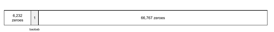
یک آرایه ۷۳۰۰۰ عنصری بسیار طولانی است. اگر یک لایه جاسازی به مدل اضافه نکنید، آموزش به دلیل ضرب ۷۲۹۹۹ صفر بسیار زمانبر خواهد بود. شاید شما لایه جاسازی را طوری انتخاب کنید که شامل ۱۲ بعد باشد. در نتیجه، لایه جاسازی به تدریج یک بردار جاسازی جدید برای هر گونه درخت یاد میگیرد.
در شرایط خاص، هش کردن جایگزین معقولی برای لایه جاسازی است.
برای اطلاعات بیشتر به دوره فشرده جاسازیها در یادگیری ماشین مراجعه کنید.
دوران
یک دوره آموزشی کامل بر روی کل مجموعه آموزشی به گونهای که هر مثال یک بار پردازش شده باشد.
یک دوره (epoch) نشان دهنده N / تعداد تکرارهای آموزشی با اندازه دسته است، که در آن N تعداد کل مثالها است.
برای مثال، موارد زیر را فرض کنید:
- مجموعه دادهها شامل ۱۰۰۰ نمونه است.
- اندازه دسته 50 نمونه است.
بنابراین، یک دوره زمانی واحد به 20 تکرار نیاز دارد:
1 epoch = (N/batch size) = (1,000 / 50) = 20 iterations
برای اطلاعات بیشتر به رگرسیون خطی: هایپرپارامترها در دوره فشرده یادگیری ماشین مراجعه کنید.
مثال
مقادیر یک ردیف از ویژگیها و احتمالاً یک برچسب . مثالها در یادگیری نظارتشده به دو دسته کلی تقسیم میشوند:
- یک مثال برچسبگذاری شده شامل یک یا چند ویژگی و یک برچسب است. مثالهای برچسبگذاری شده در طول آموزش استفاده میشوند.
- یک مثال بدون برچسب شامل یک یا چند ویژگی است اما برچسبی ندارد. مثالهای بدون برچسب در طول استنتاج استفاده میشوند.
برای مثال، فرض کنید در حال آموزش مدلی برای تعیین تأثیر شرایط آب و هوایی بر نمرات آزمون دانشآموزان هستید. در اینجا سه مثال با برچسب آورده شده است:
| ویژگیها | برچسب | ||
|---|---|---|---|
| دما | رطوبت | فشار | نمره آزمون |
| ۱۵ | ۴۷ | ۹۹۸ | خوب |
| ۱۹ | ۳۴ | ۱۰۲۰ | عالی |
| ۱۸ | ۹۲ | ۱۰۱۲ | ضعیف |
در اینجا سه مثال بدون برچسب آورده شده است:
| دما | رطوبت | فشار | |
|---|---|---|---|
| ۱۲ | ۶۲ | ۱۰۱۴ عدد | |
| ۲۱ | ۴۷ | ۱۰۱۷ عدد | |
| ۱۹ | ۴۱ | ۱۰۲۱ |
ردیف یک مجموعه داده معمولاً منبع خام برای یک مثال است. یعنی، یک مثال معمولاً شامل زیرمجموعهای از ستونهای مجموعه داده است. علاوه بر این، ویژگیهای موجود در یک مثال میتوانند شامل ویژگیهای مصنوعی مانند تقاطع ویژگیها نیز باشند.
برای اطلاعات بیشتر به آموزش نظارتشده در درس مقدمهای بر یادگیری ماشین مراجعه کنید.
ف
منفی کاذب (FN)
مثالی که در آن مدل به اشتباه کلاس منفی را پیشبینی میکند. برای مثال، مدل پیشبینی میکند که یک پیام ایمیل خاص هرزنامه (کلاس منفی) نیست ، اما آن پیام ایمیل در واقع هرزنامه است .
مثبت کاذب (FP)
مثالی که در آن مدل به اشتباه کلاس مثبت را پیشبینی میکند. برای مثال، مدل پیشبینی میکند که یک پیام ایمیل خاص هرزنامه (کلاس مثبت) است، اما آن پیام ایمیل در واقع هرزنامه نیست .
برای اطلاعات بیشتر به بخش آستانهها و ماتریس درهمریختگی در دوره فشرده یادگیری ماشین مراجعه کنید.
نرخ مثبت کاذب (FPR)
نسبت نمونههای منفی واقعی که مدل به اشتباه کلاس مثبت را برای آنها پیشبینی کرده است. فرمول زیر نرخ مثبت کاذب را محاسبه میکند:
نرخ مثبت کاذب، محور x در منحنی ROC است.
برای اطلاعات بیشتر به بخش طبقهبندی: ROC و AUC در دوره فشرده یادگیری ماشین مراجعه کنید.
ویژگی
یک متغیر ورودی به یک مدل یادگیری ماشین. یک مثال شامل یک یا چند ویژگی است. برای مثال، فرض کنید شما در حال آموزش یک مدل برای تعیین تأثیر شرایط آب و هوایی بر نمرات آزمون دانشآموزان هستید. جدول زیر سه مثال را نشان میدهد که هر کدام شامل سه ویژگی و یک برچسب هستند:
| ویژگیها | برچسب | ||
|---|---|---|---|
| دما | رطوبت | فشار | نمره آزمون |
| ۱۵ | ۴۷ | ۹۹۸ | ۹۲ |
| ۱۹ | ۳۴ | ۱۰۲۰ | ۸۴ |
| ۱۸ | ۹۲ | ۱۰۱۲ | ۸۷ |
با برچسب تضاد ایجاد کنید.
برای اطلاعات بیشتر به آموزش نظارتشده در درس مقدمهای بر یادگیری ماشین مراجعه کنید.
صلیب ویژگی
یک ویژگی مصنوعی که با "تقاطع" ویژگیهای طبقهبندیشده یا سطلی شکل گرفته است.
برای مثال، یک مدل «پیشبینی خلق و خو» را در نظر بگیرید که دما را در یکی از چهار دسته زیر نشان میدهد:
-
freezing -
chilly -
temperate -
warm
و سرعت باد را در یکی از سه حالت زیر نشان میدهد:
-
still -
light -
windy
بدون تقاطع ویژگیها، مدل خطی به طور مستقل روی هر یک از هفت سطل مختلف قبلی آموزش میبیند. بنابراین، مدل به طور مستقل روی مثلاً freezing آموزش میبیند، فارغ از آموزش روی مثلاً windy .
به عنوان یک روش جایگزین، میتوانید یک تقاطع ویژگی از دما و سرعت باد ایجاد کنید. این ویژگی مصنوعی میتواند ۱۲ مقدار ممکن زیر را داشته باشد:
-
freezing-still -
freezing-light -
freezing-windy -
chilly-still -
chilly-light -
chilly-windy -
temperate-still -
temperate-light -
temperate-windy -
warm-still -
warm-light -
warm-windy
به لطف تقاطع ویژگیها، مدل میتواند تفاوتهای خلق و خوی بین یک روز freezing-windy و یک روز freezing-still تشخیص دهد.
اگر یک ویژگی ترکیبی از دو ویژگی که هر کدام سطلهای مختلف زیادی دارند ایجاد کنید، ترکیب ویژگی حاصل تعداد بسیار زیادی ترکیب ممکن خواهد داشت. برای مثال، اگر یک ویژگی ۱۰۰۰ سطل و ویژگی دیگر ۲۰۰۰ سطل داشته باشد، ترکیب ویژگی حاصل ۲،۰۰۰،۰۰۰ سطل خواهد داشت.
به طور رسمی، یک ضربدر یک ضرب دکارتی است.
تقاطع ویژگیها بیشتر با مدلهای خطی استفاده میشوند و به ندرت با شبکههای عصبی به کار میروند.
برای اطلاعات بیشتر به بخش «دادههای دستهبندیشده: تقاطع ویژگیها» در دوره فشرده یادگیری ماشین مراجعه کنید.
مهندسی ویژگی
فرآیندی که شامل مراحل زیر است:
- تعیین اینکه کدام ویژگیها ممکن است در آموزش یک مدل مفید باشند.
- تبدیل دادههای خام از مجموعه دادهها به نسخههای کارآمد از آن ویژگیها.
برای مثال، ممکن است تشخیص دهید که temperature میتواند یک ویژگی مفید باشد. سپس، میتوانید با استفاده از روش سطلبندی، آنچه مدل میتواند از محدودههای temperature مختلف بیاموزد را بهینهسازی کنید.
مهندسی ویژگی گاهی اوقات استخراج ویژگی یا ویژگیسازی نامیده میشود.
See Numerical data: How a model ingests data using feature vectors in Machine Learning Crash Course for more information.
feature set
The group of features your machine learning model trains on. For example, a simple feature set for a model that predicts housing prices might consist of postal code, property size, and property condition.
feature vector
The array of feature values comprising an example . The feature vector is input during training and during inference . For example, the feature vector for a model with two discrete features might be:
[0.92, 0.56]

Each example supplies different values for the feature vector, so the feature vector for the next example could be something like:
[0.73, 0.49]
Feature engineering determines how to represent features in the feature vector. For example, a binary categorical feature with five possible values might be represented with one-hot encoding . In this case, the portion of the feature vector for a particular example would consist of four zeroes and a single 1.0 in the third position, as follows:
[0.0, 0.0, 1.0, 0.0, 0.0]
As another example, suppose your model consists of three features:
- a binary categorical feature with five possible values represented with one-hot encoding; for example:
[0.0, 1.0, 0.0, 0.0, 0.0] - another binary categorical feature with three possible values represented with one-hot encoding; for example:
[0.0, 0.0, 1.0] - a floating-point feature; for example:
8.3.
In this case, the feature vector for each example would be represented by nine values. Given the example values in the preceding list, the feature vector would be:
0.0
1.0
0.0
0.0
0.0
0.0
0.0
1.0
8.3
See Numerical data: How a model ingests data using feature vectors in Machine Learning Crash Course for more information.
feedback loop
In machine learning, a situation in which a model's predictions influence the training data for the same model or another model. For example, a model that recommends movies will influence the movies that people see, which will then influence subsequent movie recommendation models.
See Production ML systems: Questions to ask in Machine Learning Crash Course for more information.
جی
تعمیم
A model's ability to make correct predictions on new, previously unseen data. A model that can generalize is the opposite of a model that is overfitting .
See Generalization in Machine Learning Crash Course for more information.
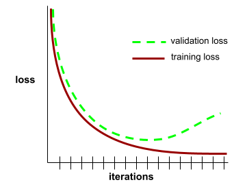
generalization curve
A plot of both training loss and validation loss as a function of the number of iterations .
A generalization curve can help you detect possible overfitting . For example, the following generalization curve suggests overfitting because validation loss ultimately becomes significantly higher than training loss.
See Generalization in Machine Learning Crash Course for more information.
gradient descent
A mathematical technique to minimize loss . Gradient descent iteratively adjusts weights and biases , gradually finding the best combination to minimize loss.
Gradient descent is older—much, much older—than machine learning.
See the Linear regression: Gradient descent in Machine Learning Crash Course for more information.
ground truth
Reality.
The thing that actually happened.
For example, consider a binary classification model that predicts whether a student in their first year of university will graduate within six years. Ground truth for this model is whether or not that student actually graduated within six years.
ح
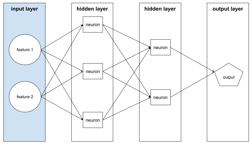
hidden layer
A layer in a neural network between the input layer (the features) and the output layer (the prediction). Each hidden layer consists of one or more neurons . For example, the following neural network contains two hidden layers, the first with three neurons and the second with two neurons:
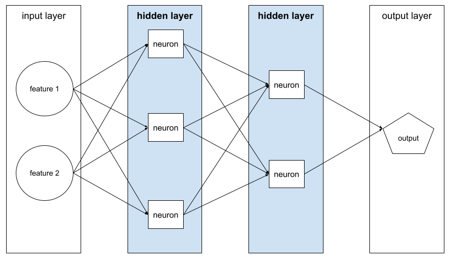
A deep neural network contains more than one hidden layer. For example, the preceding illustration is a deep neural network because the model contains two hidden layers.
See Neural networks: Nodes and hidden layers in Machine Learning Crash Course for more information.
hyperparameter
The variables that you or a hyperparameter tuning serviceadjust during successive runs of training a model. For example, learning rate is a hyperparameter. You could set the learning rate to 0.01 before one training session. If you determine that 0.01 is too high, you could perhaps set the learning rate to 0.003 for the next training session.
In contrast, parameters are the various weights and bias that the model learns during training.
See Linear regression: Hyperparameters in Machine Learning Crash Course for more information.
من
independently and identically distributed (iid)
Data drawn from a distribution that doesn't change, and where each value drawn doesn't depend on values that have been drawn previously. An iid is the ideal gas of machine learning—a useful mathematical construct but almost never exactly found in the real world. For example, the distribution of visitors to a web page may be iid over a brief window of time; that is, the distribution doesn't change during that brief window and one person's visit is generally independent of another's visit. However, if you expand that window of time, seasonal differences in the web page's visitors may appear.
See also nonstationarity .
استنباط
در یادگیری ماشین سنتی، فرآیند انجام پیشبینیها با اعمال یک مدل آموزشدیده بر روی نمونههای بدون برچسب . برای کسب اطلاعات بیشتر به یادگیری نظارتشده در دوره مقدماتی یادگیری ماشین مراجعه کنید.
در مدلهای زبانی بزرگ ، استنتاج فرآیند استفاده از یک مدل آموزشدیده برای تولید پاسخ به یک ورودی فوری است.
استنباط در آمار معنای تا حدودی متفاوتی دارد. برای جزئیات بیشتر به مقاله ویکی پدیا در مورد استنباط آماری مراجعه کنید.
input layer
The layer of a neural network that holds the feature vector . That is, the input layer provides examples for training or inference . For example, the input layer in the following neural network consists of two features:
تفسیرپذیری
The ability to explain or to present an ML model's reasoning in understandable terms to a human.
Most linear regression models, for example, are highly interpretable. (You merely need to look at the trained weights for each feature.) Decision forests are also highly interpretable. Some models, however, require sophisticated visualization to become interpretable.
You can use the Learning Interpretability Tool (LIT) to interpret ML models.
تکرار
A single update of a model's parameters—the model's weights and biases —during training . The batch size determines how many examples the model processes in a single iteration. For instance, if the batch size is 20, then the model processes 20 examples before adjusting the parameters.
When training a neural network , a single iteration involves the following two passes:
- A forward pass to evaluate loss on a single batch.
- A backward pass ( backpropagation ) to adjust the model's parameters based on the loss and the learning rate.
See Gradient descent in Machine Learning Crash Course for more information.
ل
L 0 regularization
A type of regularization that penalizes the total number of nonzero weights in a model. For example, a model having 11 nonzero weights would be penalized more than a similar model having 10 nonzero weights.
L 0 regularization is sometimes called L0-norm regularization .
L 1 loss
A loss function that calculates the absolute value of the difference between actual label values and the values that a model predicts. For example, here's the calculation of L 1 loss for a batch of five examples :
| Actual value of example | Model's predicted value | Absolute value of delta |
|---|---|---|
| ۷ | ۶ | ۱ |
| ۵ | ۴ | ۱ |
| ۸ | ۱۱ | ۳ |
| ۴ | ۶ | ۲ |
| ۹ | ۸ | ۱ |
| 8 = L 1 loss | ||
L 1 loss is less sensitive to outliers than L 2 loss .
The Mean Absolute Error is the average L 1 loss per example.
See Linear regression: Loss in Machine Learning Crash Course for more information.
L 1 regularization
A type of regularization that penalizes weights in proportion to the sum of the absolute value of the weights. L 1 regularization helps drive the weights of irrelevant or barely relevant features to exactly 0 . A feature with a weight of 0 is effectively removed from the model.
Contrast with L 2 regularization .
L 2 loss
A loss function that calculates the square of the difference between actual label values and the values that a model predicts. For example, here's the calculation of L 2 loss for a batch of five examples :
| Actual value of example | Model's predicted value | Square of delta |
|---|---|---|
| ۷ | ۶ | ۱ |
| ۵ | ۴ | ۱ |
| ۸ | ۱۱ | ۹ |
| ۴ | ۶ | ۴ |
| ۹ | ۸ | ۱ |
| 16 = L 2 loss | ||
Due to squaring, L 2 loss amplifies the influence of outliers . That is, L 2 loss reacts more strongly to bad predictions than L 1 loss . For example, the L 1 loss for the preceding batch would be 8 rather than 16. Notice that a single outlier accounts for 9 of the 16.
Regression models typically use L 2 loss as the loss function.
The Mean Squared Error is the average L 2 loss per example. Squared loss is another name for L 2 loss.
See Logistic regression: Loss and regularization in Machine Learning Crash Course for more information.
L 2 regularization
A type of regularization that penalizes weights in proportion to the sum of the squares of the weights. L 2 regularization helps drive outlier weights (those with high positive or low negative values) closer to 0 but not quite to 0 . Features with values very close to 0 remain in the model but don't influence the model's prediction very much.
L 2 regularization always improves generalization in linear models .
Contrast with L 1 regularization .
See Overfitting: L2 regularization in Machine Learning Crash Course for more information.
برچسب
In supervised machine learning , the "answer" or "result" portion of an example .
Each labeled example consists of one or more features and a label. For example, in a spam detection dataset, the label would probably be either "spam" or "not spam." In a rainfall dataset, the label might be the amount of rain that fell during a certain period.
See Supervised Learning in Introduction to Machine Learning for more information.
labeled example
An example that contains one or more features and a label . For example, the following table shows three labeled examples from a house valuation model, each with three features and one label:
| Number of bedrooms | Number of bathrooms | House age | House price (label) |
|---|---|---|---|
| ۳ | ۲ | ۱۵ | $345,000 |
| ۲ | ۱ | ۷۲ | $179,000 |
| ۴ | ۲ | ۳۴ | $392,000 |
In supervised machine learning , models train on labeled examples and make predictions on unlabeled examples .
Contrast labeled example with unlabeled examples.
See Supervised Learning in Introduction to Machine Learning for more information.
لامبدا
Synonym for regularization rate .
Lambda is an overloaded term. Here we're focusing on the term's definition within regularization .
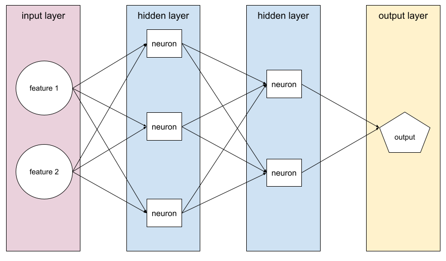
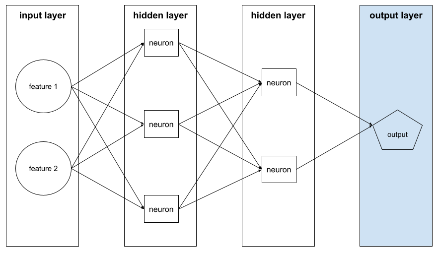
لایه
A set of neurons in a neural network . Three common types of layers are as follows:
- The input layer , which provides values for all the features .
- One or more hidden layers , which find nonlinear relationships between the features and the label.
- The output layer , which provides the prediction.
For example, the following illustration shows a neural network with one input layer, two hidden layers, and one output layer:
In TensorFlow , layers are also Python functions that take Tensors and configuration options as input and produce other tensors as output.
learning rate
A floating-point number that tells the gradient descent algorithm how strongly to adjust weights and biases on each iteration . For example, a learning rate of 0.3 would adjust weights and biases three times more powerfully than a learning rate of 0.1.
Learning rate is a key hyperparameter . If you set the learning rate too low, training will take too long. If you set the learning rate too high, gradient descent often has trouble reaching convergence .
See Linear regression: Hyperparameters in Machine Learning Crash Course for more information.
خطی
A relationship between two or more variables that can be represented solely through addition and multiplication.
The plot of a linear relationship is a line.
Contrast with nonlinear .
linear model
A model that assigns one weight per feature to make predictions . (Linear models also incorporate a bias .) In contrast, the relationship of features to predictions in deep models is generally nonlinear .
Linear models are usually easier to train and more interpretable than deep models. However, deep models can learn complex relationships between features.
Linear regression and logistic regression are two types of linear models.
رگرسیون خطی
A type of machine learning model in which both of the following are true:
- The model is a linear model .
- The prediction is a floating-point value. (This is the regression part of linear regression .)
Contrast linear regression with logistic regression . Also, contrast regression with classification .
See Linear regression in Machine Learning Crash Course for more information.
logistic regression
A type of regression model that predicts a probability. Logistic regression models have the following characteristics:
- The label is categorical . The term logistic regression usually refers to binary logistic regression , that is, to a model that calculates probabilities for labels with two possible values. A less common variant, multinomial logistic regression , calculates probabilities for labels with more than two possible values.
- The loss function during training is Log Loss . (Multiple Log Loss units can be placed in parallel for labels with more than two possible values.)
- The model has a linear architecture, not a deep neural network. However, the remainder of this definition also applies to deep models that predict probabilities for categorical labels.
For example, consider a logistic regression model that calculates the probability of an input email being either spam or not spam. During inference, suppose the model predicts 0.72. Therefore, the model is estimating:
- A 72% chance of the email being spam.
- A 28% chance of the email not being spam.
A logistic regression model uses the following two-step architecture:
- The model generates a raw prediction (y') by applying a linear function of input features.
- The model uses that raw prediction as input to a sigmoid function , which converts the raw prediction to a value between 0 and 1, exclusive.
Like any regression model, a logistic regression model predicts a number. However, this number typically becomes part of a binary classification model as follows:
- If the predicted number is greater than the classification threshold , the binary classification model predicts the positive class.
- If the predicted number is less than the classification threshold, the binary classification model predicts the negative class.
See Logistic regression in Machine Learning Crash Course for more information.
Log Loss
The loss function used in binary logistic regression .
See Logistic regression: Loss and regularization in Machine Learning Crash Course for more information.
log-odds
The logarithm of the odds of some event.
ضرر
During the training of a supervised model , a measure of how far a model's prediction is from its label .
A loss function calculates the loss.
See Linear regression: Loss in Machine Learning Crash Course for more information.
loss curve
A plot of loss as a function of the number of training iterations . The following plot shows a typical loss curve:
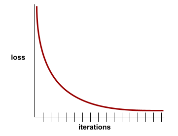
Loss curves can help you determine when your model is converging or overfitting .
Loss curves can plot all of the following types of loss:
See also generalization curve .
See Overfitting: Interpreting loss curves in Machine Learning Crash Course for more information.
loss function
During training or testing, a mathematical function that calculates the loss on a batch of examples. A loss function returns a lower loss for models that makes good predictions than for models that make bad predictions.
The goal of training is typically to minimize the loss that a loss function returns.
Many different kinds of loss functions exist. Pick the appropriate loss function for the kind of model you are building. For example:
- L 2 loss (or Mean Squared Error ) is the loss function for linear regression .
- Log Loss is the loss function for logistic regression .
م
یادگیری ماشینی
A program or system that trains a model from input data. The trained model can make useful predictions from new (never-before-seen) data drawn from the same distribution as the one used to train the model.
Machine learning also refers to the field of study concerned with these programs or systems.
See the Introduction to Machine Learning course for more information.
majority class
The more common label in a class-imbalanced dataset . For example, given a dataset containing 99% negative labels and 1% positive labels, the negative labels are the majority class.
Contrast with minority class .
See Datasets: Imbalanced datasets in Machine Learning Crash Course for more information.
mini-batch
A small, randomly selected subset of a batch processed in one iteration . The batch size of a mini-batch is usually between 10 and 1,000 examples.
For example, suppose the entire training set (the full batch) consists of 1,000 examples. Further suppose that you set the batch size of each mini-batch to 20. Therefore, each iteration determines the loss on a random 20 of the 1,000 examples and then adjusts the weights and biases accordingly.
It is much more efficient to calculate the loss on a mini-batch than the loss on all the examples in the full batch.
See Linear regression: Hyperparameters in Machine Learning Crash Course for more information.
minority class
The less common label in a class-imbalanced dataset . For example, given a dataset containing 99% negative labels and 1% positive labels, the positive labels are the minority class.
Contrast with majority class .
See Datasets: Imbalanced datasets in Machine Learning Crash Course for more information.
مدل
In general, any mathematical construct that processes input data and returns output. Phrased differently, a model is the set of parameters and structure needed for a system to make predictions. In supervised machine learning , a model takes an example as input and infers a prediction as output. Within supervised machine learning, models differ somewhat. For example:
- A linear regression model consists of a set of weights and a bias .
- A neural network model consists of:
- A set of hidden layers , each containing one or more neurons .
- The weights and bias associated with each neuron.
- A decision tree model consists of:
- The shape of the tree; that is, the pattern in which the conditions and leaves are connected.
- The conditions and leaves.
You can save, restore, or make copies of a model.
Unsupervised machine learning also generates models, typically a function that can map an input example to the most appropriate cluster .
multi-class classification
In supervised learning, a classification problem in which the dataset contains more than two classes of labels. For example, the labels in the Iris dataset must be one of the following three classes:
- Iris setosa
- Iris virginica
- Iris versicolor
A model trained on the Iris dataset that predicts Iris type on new examples is performing multi-class classification.
In contrast, classification problems that distinguish between exactly two classes are binary classification models . For example, an email model that predicts either spam or not spam is a binary classification model.
In clustering problems, multi-class classification refers to more than two clusters.
See Neural networks: Multi-class classification in Machine Learning Crash Course for more information.
ن
negative class
In binary classification , one class is termed positive and the other is termed negative . The positive class is the thing or event that the model is testing for and the negative class is the other possibility. For example:
- The negative class in a medical test might be "not tumor."
- The negative class in an email classification model might be "not spam."
Contrast with positive class .
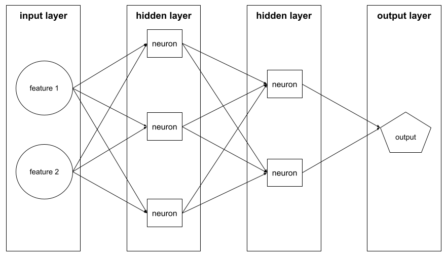
neural network
A model containing at least one hidden layer . A deep neural network is a type of neural network containing more than one hidden layer. For example, the following diagram shows a deep neural network containing two hidden layers.
Each neuron in a neural network connects to all of the nodes in the next layer. For example, in the preceding diagram, notice that each of the three neurons in the first hidden layer separately connect to both of the two neurons in the second hidden layer.
Neural networks implemented on computers are sometimes called artificial neural networks to differentiate them from neural networks found in brains and other nervous systems.
Some neural networks can mimic extremely complex nonlinear relationships between different features and the label.
See also convolutional neural network and recurrent neural network .
See Neural networks in Machine Learning Crash Course for more information.
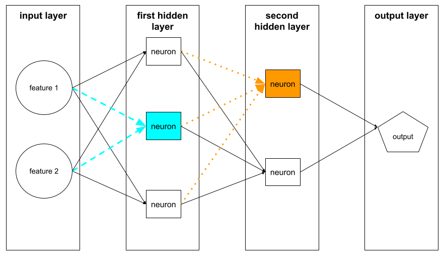
نورون
In machine learning, a distinct unit within a hidden layer of a neural network . Each neuron performs the following two-step action:
- Calculates the weighted sum of input values multiplied by their corresponding weights.
- Passes the weighted sum as input to an activation function .
A neuron in the first hidden layer accepts inputs from the feature values in the input layer . A neuron in any hidden layer beyond the first accepts inputs from the neurons in the preceding hidden layer. For example, a neuron in the second hidden layer accepts inputs from the neurons in the first hidden layer.
The following illustration highlights two neurons and their inputs.
A neuron in a neural network mimics the behavior of neurons in brains and other parts of nervous systems.
node (neural network)
A neuron in a hidden layer .
See Neural Networks in Machine Learning Crash Course for more information.
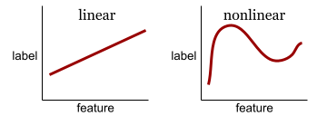
غیرخطی
A relationship between two or more variables that can't be represented solely through addition and multiplication. A linear relationship can be represented as a line; a nonlinear relationship can't be represented as a line. For example, consider two models that each relate a single feature to a single label. The model on the left is linear and the model on the right is nonlinear:
See Neural networks: Nodes and hidden layers in Machine Learning Crash Course to experiment with different kinds of nonlinear functions.
nonstationarity
A feature whose values change across one or more dimensions, usually time. For example, consider the following examples of nonstationarity:
- The number of swimsuits sold at a particular store varies with the season.
- The quantity of a particular fruit harvested in a particular region is zero for much of the year but large for a brief period.
- Due to climate change, annual mean temperatures are shifting.
Contrast with stationarity .
normalization
Broadly speaking, the process of converting a variable's actual range of values into a standard range of values, such as:
- -1 to +1
- 0 to 1
- Z-scores (roughly, -3 to +3)
For example, suppose the actual range of values of a certain feature is 800 to 2,400. As part of feature engineering , you could normalize the actual values down to a standard range, such as -1 to +1.
Normalization is a common task in feature engineering . Models usually train faster (and produce better predictions) when every numerical feature in the feature vector has roughly the same range.
See also Z-score normalization .
See Numerical Data: Normalization in Machine Learning Crash Course for more information.
numerical data
Features represented as integers or real-valued numbers. For example, a house valuation model would probably represent the size of a house (in square feet or square meters) as numerical data. Representing a feature as numerical data indicates that the feature's values have a mathematical relationship to the label. That is, the number of square meters in a house probably has some mathematical relationship to the value of the house.
Not all integer data should be represented as numerical data. For example, postal codes in some parts of the world are integers; however, integer postal codes shouldn't be represented as numerical data in models. That's because a postal code of 20000 is not twice (or half) as potent as a postal code of 10000. Furthermore, although different postal codes do correlate to different real estate values, we can't assume that real estate values at postal code 20000 are twice as valuable as real estate values at postal code 10000. Postal codes should be represented as categorical data instead.
Numerical features are sometimes called continuous features .
See Working with numerical data in Machine Learning Crash Course for more information.
ای
آفلاین
Synonym for static .
offline inference
The process of a model generating a batch of predictions and then caching (saving) those predictions. Apps can then access the inferred prediction from the cache rather than rerunning the model.
For example, consider a model that generates local weather forecasts (predictions) once every four hours. After each model run, the system caches all the local weather forecasts. Weather apps retrieve the forecasts from the cache.
Offline inference is also called static inference .
Contrast with online inference . See Production ML systems: Static versus dynamic inference in Machine Learning Crash Course for more information.
one-hot encoding
Representing categorical data as a vector in which:
- One element is set to 1.
- All other elements are set to 0.
One-hot encoding is commonly used to represent strings or identifiers that have a finite set of possible values. For example, suppose a certain categorical feature named Scandinavia has five possible values:
- "Denmark"
- "Sweden"
- "Norway"
- "Finland"
- "Iceland"
One-hot encoding could represent each of the five values as follows:
| کشور | بردار | ||||
|---|---|---|---|---|---|
| "Denmark" | ۱ | 0 | 0 | 0 | 0 |
| "Sweden" | 0 | ۱ | 0 | 0 | 0 |
| "Norway" | 0 | 0 | ۱ | 0 | 0 |
| "Finland" | 0 | 0 | 0 | ۱ | 0 |
| "Iceland" | 0 | 0 | 0 | 0 | ۱ |
Thanks to one-hot encoding, a model can learn different connections based on each of the five countries.
Representing a feature as numerical data is an alternative to one-hot encoding. Unfortunately, representing the Scandinavian countries numerically is not a good choice. For example, consider the following numeric representation:
- "Denmark" is 0
- "Sweden" is 1
- "Norway" is 2
- "Finland" is 3
- "Iceland" is 4
With numeric encoding, a model would interpret the raw numbers mathematically and would try to train on those numbers. However, Iceland isn't actually twice as much (or half as much) of something as Norway, so the model would come to some strange conclusions.
See Categorical data: Vocabulary and one-hot encoding in Machine Learning Crash Course for more information.
one-vs.-all
Given a classification problem with N classes, a solution consisting of N separate binary classification model—one binary classification model for each possible outcome. For example, given a model that classifies examples as animal, vegetable, or mineral, a one-vs.-all solution would provide the following three separate binary classification models:
- animal versus not animal
- vegetable versus not vegetable
- mineral versus not mineral
آنلاین
Synonym for dynamic .
online inference
Generating predictions on demand. For example, suppose an app passes input to a model and issues a request for a prediction. A system using online inference responds to the request by running the model (and returning the prediction to the app).
Contrast with offline inference .
See Production ML systems: Static versus dynamic inference in Machine Learning Crash Course for more information.
output layer
The "final" layer of a neural network. The output layer contains the prediction.
The following illustration shows a small deep neural network with an input layer, two hidden layers, and an output layer:
بیشبرازش
Creating a model that matches the training data so closely that the model fails to make correct predictions on new data.
Regularization can reduce overfitting. Training on a large and diverse training set can also reduce overfitting.
See Overfitting in Machine Learning Crash Course for more information.
پ
پانداها
A column-oriented data analysis API built on top of numpy . Many machine learning frameworks, including TensorFlow, support pandas data structures as inputs. See the pandas documentation for details.
پارامتر
The weights and biases that a model learns during training . For example, in a linear regression model, the parameters consist of the bias ( b ) and all the weights ( w 1 , w 2 , and so on) in the following formula:
In contrast, hyperparameters are the values that you (or a hyperparameter tuning service) supply to the model. For example, learning rate is a hyperparameter.
positive class
The class you are testing for.
For example, the positive class in a cancer model might be "tumor." The positive class in an email classification model might be "spam."
Contrast with negative class .
post-processing
Adjusting the output of a model after the model has been run. Post-processing can be used to enforce fairness constraints without modifying models themselves.
For example, one might apply post-processing to a binary classification model by setting a classification threshold such that equality of opportunity is maintained for some attribute by checking that the true positive rate is the same for all values of that attribute.
precision
A metric for classification models that answers the following question:
When the model predicted the positive class , what percentage of the predictions were correct?
Here is the formula:
where:
- true positive means the model correctly predicted the positive class.
- false positive means the model mistakenly predicted the positive class.
For example, suppose a model made 200 positive predictions. Of these 200 positive predictions:
- 150 were true positives.
- 50 were false positives.
In this case:
Contrast with accuracy and recall .
See Classification: Accuracy, recall, precision and related metrics in Machine Learning Crash Course for more information.
پیشبینی
A model's output. For example:
- The prediction of a binary classification model is either the positive class or the negative class.
- The prediction of a multi-class classification model is one class.
- The prediction of a linear regression model is a number.
proxy labels
Data used to approximate labels not directly available in a dataset.
For example, suppose you must train a model to predict employee stress level. Your dataset contains a lot of predictive features but doesn't contain a label named stress level. Undaunted, you pick "workplace accidents" as a proxy label for stress level. After all, employees under high stress get into more accidents than calm employees. Or do they? Maybe workplace accidents actually rise and fall for multiple reasons.
As a second example, suppose you want is it raining? to be a Boolean label for your dataset, but your dataset doesn't contain rain data. If photographs are available, you might establish pictures of people carrying umbrellas as a proxy label for is it raining? Is that a good proxy label? Possibly, but people in some cultures may be more likely to carry umbrellas to protect against sun than the rain.
Proxy labels are often imperfect. When possible, choose actual labels over proxy labels. That said, when an actual label is absent, pick the proxy label very carefully, choosing the least horrible proxy label candidate.
See Datasets: Labels in Machine Learning Crash Course for more information.
ر
راگ
Abbreviation for retrieval-augmented generation .
ارزیاب
A human who provides labels for examples . "Annotator" is another name for rater.
See Categorical data: Common issues in Machine Learning Crash Course for more information.
به یاد بیاورید
A metric for classification models that answers the following question:
When ground truth was the positive class , what percentage of predictions did the model correctly identify as the positive class?
Here is the formula:
\[\text{Recall} = \frac{\text{true positives}} {\text{true positives} + \text{false negatives}} \]
where:
- true positive means the model correctly predicted the positive class.
- false negative means that the model mistakenly predicted the negative class .
For instance, suppose your model made 200 predictions on examples for which ground truth was the positive class. Of these 200 predictions:
- 180 were true positives.
- 20 were false negatives.
In this case:
\[\text{Recall} = \frac{\text{180}} {\text{180} + \text{20}} = 0.9 \]
See Classification: Accuracy, recall, precision and related metrics for more information.
Rectified Linear Unit (ReLU)
An activation function with the following behavior:
- If input is negative or zero, then the output is 0.
- If input is positive, then the output is equal to the input.
برای مثال:
- If the input is -3, then the output is 0.
- If the input is +3, then the output is 3.0.
Here is a plot of ReLU:
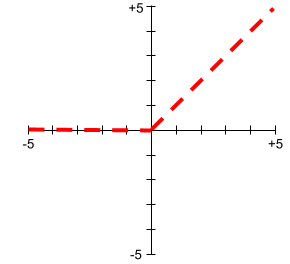
ReLU is a very popular activation function. Despite its simple behavior, ReLU still enables a neural network to learn nonlinear relationships between features and the label .
regression model
Informally, a model that generates a numerical prediction. (In contrast, a classification model generates a class prediction.) For example, the following are all regression models:
- A model that predicts a certain house's value in Euros, such as 423,000.
- A model that predicts a certain tree's life expectancy in years, such as 23.2.
- A model that predicts the amount of rain in inches that will fall in a certain city over the next six hours, such as 0.18.
Two common types of regression models are:
- Linear regression , which finds the line that best fits label values to features.
- Logistic regression , which generates a probability between 0.0 and 1.0 that a system typically then maps to a class prediction.
Not every model that outputs numerical predictions is a regression model. In some cases, a numeric prediction is really just a classification model that happens to have numeric class names. For example, a model that predicts a numeric postal code is a classification model, not a regression model.
منظم سازی
Any mechanism that reduces overfitting . Popular types of regularization include:
- L 1 regularization
- L 2 regularization
- dropout regularization
- early stopping (this is not a formal regularization method, but can effectively limit overfitting)
Regularization can also be defined as the penalty on a model's complexity.
See Overfitting: Model complexity in Machine Learning Crash Course for more information.
regularization rate
A number that specifies the relative importance of regularization during training. Raising the regularization rate reduces overfitting but may reduce the model's predictive power. Conversely, reducing or omitting the regularization rate increases overfitting.
See Overfitting: L2 regularization in Machine Learning Crash Course for more information.
ReLU
Abbreviation for Rectified Linear Unit .
retrieval-augmented generation (RAG)
A technique for improving the quality of large language model (LLM) output by grounding it with sources of knowledge retrieved after the model was trained. RAG improves the accuracy of LLM responses by providing the trained LLM with access to information retrieved from trusted knowledge bases or documents.
Common motivations to use retrieval-augmented generation include:
- Increasing the factual accuracy of a model's generated responses.
- Giving the model access to knowledge it was not trained on.
- Changing the knowledge that the model uses.
- Enabling the model to cite sources.
For example, suppose that a chemistry app uses the PaLM API to generate summaries related to user queries. When the app's backend receives a query, the backend:
- Searches for ("retrieves") data that's relevant to the user's query.
- Appends ("augments") the relevant chemistry data to the user's query.
- Instructs the LLM to create a summary based on the appended data.
ROC (receiver operating characteristic) Curve
A graph of true positive rate versus false positive rate for different classification thresholds in binary classification.
The shape of an ROC curve suggests a binary classification model's ability to separate positive classes from negative classes. Suppose, for example, that a binary classification model perfectly separates all the negative classes from all the positive classes:
The ROC curve for the preceding model looks as follows:
In contrast, the following illustration graphs the raw logistic regression values for a terrible model that can't separate negative classes from positive classes at all:
The ROC curve for this model looks as follows:
Meanwhile, back in the real world, most binary classification models separate positive and negative classes to some degree, but usually not perfectly. So, a typical ROC curve falls somewhere between the two extremes:
The point on an ROC curve closest to (0.0,1.0) theoretically identifies the ideal classification threshold. However, several other real-world issues influence the selection of the ideal classification threshold. For example, perhaps false negatives cause far more pain than false positives.
A numerical metric called AUC summarizes the ROC curve into a single floating-point value.
Root Mean Squared Error (RMSE)
The square root of the Mean Squared Error .
س
تابع سیگموئید
A mathematical function that "squishes" an input value into a constrained range, typically 0 to 1 or -1 to +1. That is, you can pass any number (two, a million, negative billion, whatever) to a sigmoid and the output will still be in the constrained range. A plot of the sigmoid activation function looks as follows:
The sigmoid function has several uses in machine learning, including:
- Converting the raw output of a logistic regression or multinomial regression model to a probability.
- Acting as an activation function in some neural networks.
softmax
A function that determines probabilities for each possible class in a multi-class classification model . The probabilities add up to exactly 1.0. For example, the following table shows how softmax distributes various probabilities:
| Image is a... | احتمال |
|---|---|
| سگ | .85 |
| گربه | .13 |
| اسب | .02 |
Softmax is also called full softmax .
Contrast with candidate sampling .
See Neural networks: Multi-class classification in Machine Learning Crash Course for more information.
sparse feature
A feature whose values are predominately zero or empty. For example, a feature containing a single 1 value and a million 0 values is sparse. In contrast, a dense feature has values that are predominantly not zero or empty.
In machine learning, a surprising number of features are sparse features. Categorical features are usually sparse features. For example, of the 300 possible tree species in a forest, a single example might identify just a maple tree . Or, of the millions of possible videos in a video library, a single example might identify just "Casablanca."
In a model, you typically represent sparse features with one-hot encoding . If the one-hot encoding is big, you might put an embedding layer on top of the one-hot encoding for greater efficiency.
sparse representation
Storing only the position(s) of nonzero elements in a sparse feature.
For example, suppose a categorical feature named species identifies the 36 tree species in a particular forest. Further assume that each example identifies only a single species.
You could use a one-hot vector to represent the tree species in each example. A one-hot vector would contain a single 1 (to represent the particular tree species in that example) and 35 0 s (to represent the 35 tree species not in that example). So, the one-hot representation of maple might look something like the following:
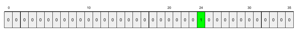
Alternatively, sparse representation would simply identify the position of the particular species. If maple is at position 24, then the sparse representation of maple would simply be:
24
Notice that the sparse representation is much more compact than the one-hot representation.
Click the icon for a slightly more complex example.
Suppose each example in your model must represent the words—but not the order of those words—in an English sentence. English consists of about 170,000 words, so English is a categorical feature with about 170,000 elements. Most English sentences use an extremely tiny fraction of those 170,000 words, so the set of words in a single example is almost certainly going to be sparse data.
Consider the following sentence:
My dog is a great dog
You could use a variant of one-hot vector to represent the words in this sentence. In this variant, multiple cells in the vector can contain a nonzero value. Furthermore, in this variant, a cell can contain an integer other than one. Although the words "my", "is", "a", and "great" appear only once in the sentence, the word "dog" appears twice. Using this variant of one-hot vectors to represent the words in this sentence yields the following 170,000-element vector:
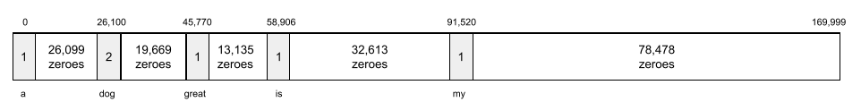
A sparse representation of the same sentence would simply be:
0: 1
26100: 2
45770: 1
58906: 1
91520: 1
See Working with categorical data in Machine Learning Crash Course for more information.
sparse vector
A vector whose values are mostly zeroes. See also sparse feature and sparsity .
squared loss
Synonym for L 2 loss .
استاتیک
Something done once rather than continuously. The terms static and offline are synonyms. The following are common uses of static and offline in machine learning:
- static model (or offline model ) is a model trained once and then used for a while.
- static training (or offline training ) is the process of training a static model.
- static inference (or offline inference ) is a process in which a model generates a batch of predictions at a time.
Contrast with dynamic .
static inference
Synonym for offline inference .
ایستایی
A feature whose values don't change across one or more dimensions, usually time. For example, a feature whose values look about the same in 2021 and 2023 exhibits stationarity.
In the real world, very few features exhibit stationarity. Even features synonymous with stability (like sea level) change over time.
Contrast with nonstationarity .
stochastic gradient descent (SGD)
A gradient descent algorithm in which the batch size is one. In other words, SGD trains on a single example chosen uniformly at random from a training set .
See Linear regression: Hyperparameters in Machine Learning Crash Course for more information.
یادگیری ماشینی تحت نظارت
Training a model from features and their corresponding labels . Supervised machine learning is analogous to learning a subject by studying a set of questions and their corresponding answers. After mastering the mapping between questions and answers, a student can then provide answers to new (never-before-seen) questions on the same topic.
Compare with unsupervised machine learning .
See Supervised Learning in the Introduction to ML course for more information.
synthetic feature
A feature not present among the input features, but assembled from one or more of them. Methods for creating synthetic features include the following:
- Bucketing a continuous feature into range bins.
- Creating a feature cross .
- Multiplying (or dividing) one feature value by other feature value(s) or by itself. For example, if
aandbare input features, then the following are examples of synthetic features:- آب
- یک ۲
- Applying a transcendental function to a feature value. For example, if
cis an input feature, then the following are examples of synthetic features:- sin(c)
- ln(c)
Features created by normalizing or scaling alone are not considered synthetic features.
تی
test loss
A metric representing a model's loss against the test set . When building a model , you typically try to minimize test loss. That's because a low test loss is a stronger quality signal than a low training loss or low validation loss .
A large gap between test loss and training loss or validation loss sometimes suggests that you need to increase the regularization rate .
آموزش
The process of determining the ideal parameters (weights and biases) comprising a model . During training, a system reads in examples and gradually adjusts parameters. Training uses each example anywhere from a few times to billions of times.
See Supervised Learning in the Introduction to ML course for more information.
training loss
A metric representing a model's loss during a particular training iteration. For example, suppose the loss function is Mean Squared Error . Perhaps the training loss (the Mean Squared Error) for the 10th iteration is 2.2, and the training loss for the 100th iteration is 1.9.
A loss curve plots training loss versus the number of iterations. A loss curve provides the following hints about training:
- A downward slope implies that the model is improving.
- An upward slope implies that the model is getting worse.
- A flat slope implies that the model has reached convergence .
For example, the following somewhat idealized loss curve shows:
- A steep downward slope during the initial iterations, which implies rapid model improvement.
- A gradually flattening (but still downward) slope until close to the end of training, which implies continued model improvement at a somewhat slower pace then during the initial iterations.
- A flat slope towards the end of training, which suggests convergence.

Although training loss is important, see also generalization .
training-serving skew
The difference between a model's performance during training and that same model's performance during serving .
training set
The subset of the dataset used to train a model .
Traditionally, examples in the dataset are divided into the following three distinct subsets:
- a training set
- a validation set
- a test set
Ideally, each example in the dataset should belong to only one of the preceding subsets. For example, a single example shouldn't belong to both the training set and the validation set.
See Datasets: Dividing the original dataset in Machine Learning Crash Course for more information.
true negative (TN)
An example in which the model correctly predicts the negative class . For example, the model infers that a particular email message is not spam , and that email message really is not spam .
true positive (TP)
An example in which the model correctly predicts the positive class . For example, the model infers that a particular email message is spam, and that email message really is spam.
true positive rate (TPR)
Synonym for recall . That is:
True positive rate is the y-axis in an ROC curve .
یو
underfitting
Producing a model with poor predictive ability because the model hasn't fully captured the complexity of the training data. Many problems can cause underfitting, including:
- Training on the wrong set of features .
- Training for too few epochs or at too low a learning rate .
- Training with too high a regularization rate .
- Providing too few hidden layers in a deep neural network.
See Overfitting in Machine Learning Crash Course for more information.
unlabeled example
An example that contains features but no label . For example, the following table shows three unlabeled examples from a house valuation model, each with three features but no house value:
| Number of bedrooms | Number of bathrooms | House age |
|---|---|---|
| ۳ | ۲ | ۱۵ |
| ۲ | ۱ | ۷۲ |
| ۴ | ۲ | ۳۴ |
In supervised machine learning , models train on labeled examples and make predictions on unlabeled examples .
In semi-supervised and unsupervised learning, unlabeled examples are used during training.
Contrast unlabeled example with labeled example .
unsupervised machine learning
Training a model to find patterns in a dataset, typically an unlabeled dataset.
The most common use of unsupervised machine learning is to cluster data into groups of similar examples. For example, an unsupervised machine learning algorithm can cluster songs based on various properties of the music. The resulting clusters can become an input to other machine learning algorithms (for example, to a music recommendation service). Clustering can help when useful labels are scarce or absent. For example, in domains such as anti-abuse and fraud, clusters can help humans better understand the data.
Contrast with supervised machine learning .
See What is Machine Learning? in the Introduction to ML course for more information.
پنجم
اعتبارسنجی
The initial evaluation of a model's quality. Validation checks the quality of a model's predictions against the validation set .
Because the validation set differs from the training set , validation helps guard against overfitting .
You might think of evaluating the model against the validation set as the first round of testing and evaluating the model against the test set as the second round of testing.
validation loss
A metric representing a model's loss on the validation set during a particular iteration of training.
See also generalization curve .
validation set
The subset of the dataset that performs initial evaluation against a trained model . Typically, you evaluate the trained model against the validation set several times before evaluating the model against the test set .
Traditionally, you divide the examples in the dataset into the following three distinct subsets:
- a training set
- a validation set
- a test set
Ideally, each example in the dataset should belong to only one of the preceding subsets. For example, a single example shouldn't belong to both the training set and the validation set.
See Datasets: Dividing the original dataset in Machine Learning Crash Course for more information.
دبلیو
وزن
A value that a model multiplies by another value. Training is the process of determining a model's ideal weights; inference is the process of using those learned weights to make predictions.
See Linear regression in Machine Learning Crash Course for more information.
weighted sum
The sum of all the relevant input values multiplied by their corresponding weights. For example, suppose the relevant inputs consist of the following:
| input value | input weight |
| ۲ | -1.3 |
| -1 | ۰.۶ |
| ۳ | 0.4 |
The weighted sum is therefore:
weighted sum = (2)(-1.3) + (-1)(0.6) + (3)(0.4) = -2.0
A weighted sum is the input argument to an activation function .
ز
Z-score normalization
A scaling technique that replaces a raw feature value with a floating-point value representing the number of standard deviations from that feature's mean. For example, consider a feature whose mean is 800 and whose standard deviation is 100. The following table shows how Z-score normalization would map the raw value to its Z-score:
| Raw value | Z-score |
|---|---|
| ۸۰۰ | 0 |
| ۹۵۰ | +1.5 |
| ۵۷۵ | -۲.۲۵ |
The machine learning model then trains on the Z-scores for that feature instead of on the raw values.
See Numerical data: Normalization in Machine Learning Crash Course for more information.