Machine Learning Glossary: Image Models

This page contains Image Models glossary terms. For all glossary terms, click here.

A

augmented reality

#image

A technology that superimposes a computer-generated image on a user's view of the real world, thus providing a composite view.

autoencoder

#language

#image

A system that learns to extract the most important information from the input. Autoencoders are a combination of an encoder and decoder. Autoencoders rely on the following two-step process:

1. The encoder maps the input to a (typically) lossy lower-dimensional (intermediate) format.
2. The decoder builds a lossy version of the original input by mapping the lower-dimensional format to the original higher-dimensional input format.

Autoencoders are trained end-to-end by having the decoder attempt to reconstruct the original input from the encoder's intermediate format as closely as possible. Because the intermediate format is smaller (lower-dimensional) than the original format, the autoencoder is forced to learn what information in the input is essential, and the output won't be perfectly identical to the input.

For example:

• If the input data is a graphic, the non-exact copy would be similar to the original graphic, but somewhat modified. Perhaps the non-exact copy removes noise from the original graphic or fills in some missing pixels.
• If the input data is text, an autoencoder would generate new text that mimics (but is not identical to) the original text.

See also variational autoencoders.

auto-regressive model

#language

#image

#generativeAI

A model that infers a prediction based on its own previous predictions. For example, auto-regressive language models predict the next token based on the previously predicted tokens. All Transformer-based large language models are auto-regressive.

In contrast, GAN-based image models are usually not auto-regressive since they generate an image in a single forward-pass and not iteratively in steps. However, certain image generation models are auto-regressive because they generate an image in steps.

B

bounding box

#image

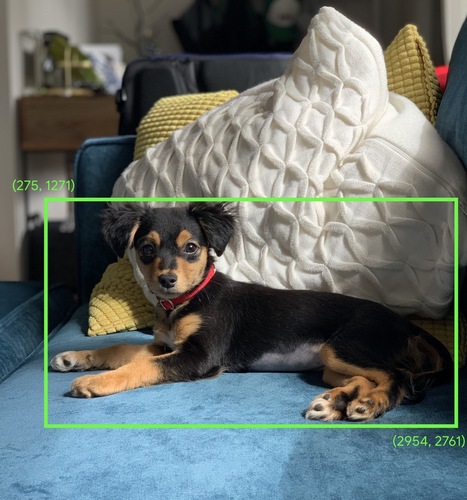
In an image, the (x, y) coordinates of a rectangle around an area of interest, such as the dog in the image below.

C

convolution

#image

In mathematics, casually speaking, a mixture of two functions. In machine learning, a convolution mixes the convolutional filter and the input matrix in order to train weights.

The term "convolution" in machine learning is often a shorthand way of referring to either convolutional operation or convolutional layer.

Without convolutions, a machine learning algorithm would have to learn a separate weight for every cell in a large tensor. For example, a machine learning algorithm training on 2K x 2K images would be forced to find 4M separate weights. Thanks to convolutions, a machine learning algorithm only has to find weights for every cell in the convolutional filter, dramatically reducing the memory needed to train the model. When the convolutional filter is applied, it is simply replicated across cells such that each is multiplied by the filter.

See Introducing Convolutional Neural Networks in the Image Classification course for more information.

convolutional filter

#image

One of the two actors in a convolutional operation. (The other actor is a slice of an input matrix.) A convolutional filter is a matrix having the same rank as the input matrix, but a smaller shape. For example, given a 28x28 input matrix, the filter could be any 2D matrix smaller than 28x28.

In photographic manipulation, all the cells in a convolutional filter are typically set to a constant pattern of ones and zeroes. In machine learning, convolutional filters are typically seeded with random numbers and then the network trains the ideal values.

See Convolution in the Image Classification course for more information.

convolutional layer

#image

A layer of a deep neural network in which a convolutional filter passes along an input matrix. For example, consider the following 3x3 convolutional filter:

The following animation shows a convolutional layer consisting of 9 convolutional operations involving the 5x5 input matrix. Notice that each convolutional operation works on a different 3x3 slice of the input matrix. The resulting 3x3 matrix (on the right) consists of the results of the 9 convolutional operations:

See Fully Connected Layers in the Image Classification course for more information.

convolutional neural network

#image

A neural network in which at least one layer is a convolutional layer. A typical convolutional neural network consists of some combination of the following layers:

• convolutional layers
• pooling layers
• dense layers

Convolutional neural networks have had great success in certain kinds of problems, such as image recognition.

convolutional operation

#image

The following two-step mathematical operation:

1. Element-wise multiplication of the convolutional filter and a slice of an input matrix. (The slice of the input matrix has the same rank and size as the convolutional filter.)
2. Summation of all the values in the resulting product matrix.

For example, consider the following 5x5 input matrix:

Now imagine the following 2x2 convolutional filter:

Each convolutional operation involves a single 2x2 slice of the input matrix. For example, suppose we use the 2x2 slice at the top-left of the input matrix. So, the convolution operation on this slice looks as follows:

A convolutional layer consists of a series of convolutional operations, each acting on a different slice of the input matrix.

D

data augmentation

#image

Artificially boosting the range and number of training examples by transforming existing examples to create additional examples. For example, suppose images are one of your features, but your dataset doesn't contain enough image examples for the model to learn useful associations. Ideally, you'd add enough labeled images to your dataset to enable your model to train properly. If that's not possible, data augmentation can rotate, stretch, and reflect each image to produce many variants of the original picture, possibly yielding enough labeled data to enable excellent training.

depthwise separable convolutional neural network (sepCNN)

#image

A convolutional neural network architecture based on Inception, but where Inception modules are replaced with depthwise separable convolutions. Also known as Xception.

A depthwise separable convolution (also abbreviated as separable convolution) factors a standard 3D convolution into two separate convolution operations that are more computationally efficient: first, a depthwise convolution, with a depth of 1 (n ✕ n ✕ 1), and then second, a pointwise convolution, with length and width of 1 (1 ✕ 1 ✕ n).

To learn more, see Xception: Deep Learning with Depthwise Separable Convolutions.

downsampling

#image

Overloaded term that can mean either of the following:

• Reducing the amount of information in a feature in order to train a model more efficiently. For example, before training an image recognition model, downsampling high-resolution images to a lower-resolution format.
• Training on a disproportionately low percentage of over-represented class examples in order to improve model training on under-represented classes. For example, in a class-imbalanced dataset, models tend to learn a lot about the majority class and not enough about the minority class. Downsampling helps balance the amount of training on the majority and minority classes.

See Datasets: Imbalanced datasets in Machine Learning Crash Course for more information.

F

fine-tuning

#language

#image

#generativeAI

A second, task-specific training pass performed on a pre-trained model to refine its parameters for a specific use case. For example, the full training sequence for some large language models is as follows:

1. Pre-training: Train a large language model on a vast general dataset, such as all the English language Wikipedia pages.
2. Fine-tuning: Train the pre-trained model to perform a specific task, such as responding to medical queries. Fine-tuning typically involves hundreds or thousands of examples focused on the specific task.

As another example, the full training sequence for a large image model is as follows:

1. Pre-training: Train a large image model on a vast general image dataset, such as all the images in Wikimedia commons.
2. Fine-tuning: Train the pre-trained model to perform a specific task, such as generating images of orcas.

Fine-tuning can entail any combination of the following strategies:

• Modifying all of the pre-trained model's existing parameters. This is sometimes called full fine-tuning.
• Modifying only some of the pre-trained model's existing parameters (typically, the layers closest to the output layer), while keeping other existing parameters unchanged (typically, the layers closest to the input layer). See parameter-efficient tuning.
• Adding more layers, typically on top of the existing layers closest to the output layer.

Fine-tuning is a form of transfer learning. As such, fine-tuning might use a different loss function or a different model type than those used to train the pre-trained model. For example, you could fine-tune a pre-trained large image model to produce a regression model that returns the number of birds in an input image.

Compare and contrast fine-tuning with the following terms:

• distillation
• prompt-based learning

See Fine-tuning in Machine Learning Crash Course for more information.

G

Gemini

#language

#image

#generativeAI

The ecosystem comprising Google's most advanced AI. Elements of this ecosystem include:

• Various Gemini models.
• The interactive conversational interface to a Gemini model. Users type prompts and Gemini responds to those prompts.
• Various Gemini APIs.
• Various business products based on Gemini models; for example, Gemini for Google Cloud.

Gemini models

#language

#image

#generativeAI

Google's state-of-the-art Transformer-based multimodal models. Gemini models are specifically designed to integrate with agents.

Users can interact with Gemini models in a variety of ways, including through an interactive dialog interface and through SDKs.

generative AI

#language

#image

#generativeAI

An emerging transformative field with no formal definition. That said, most experts agree that generative AI models can create ("generate") content that is all of the following:

• complex
• coherent
• original

For example, a generative AI model can create sophisticated essays or images.

Some earlier technologies, including LSTMs and RNNs, can also generate original and coherent content. Some experts view these earlier technologies as generative AI, while others feel that true generative AI requires more complex output than those earlier technologies can produce.

Contrast with predictive ML.

I

image recognition

#image

A process that classifies object(s), pattern(s), or concept(s) in an image. Image recognition is also known as image classification.

For more information, see ML Practicum: Image Classification.

See the ML Practicum: Image Classification course for more information.

intersection over union (IoU)

#image

The intersection of two sets divided by their union. In machine-learning image-detection tasks, IoU is used to measure the accuracy of the model's predicted bounding box with respect to the ground-truth bounding box. In this case, the IoU for the two boxes is the ratio between the overlapping area and the total area, and its value ranges from 0 (no overlap of predicted bounding box and ground-truth bounding box) to 1 (predicted bounding box and ground-truth bounding box have the exact same coordinates).

For example, in the image below:

• The predicted bounding box (the coordinates delimiting where the model predicts the night table in the painting is located) is outlined in purple.
• The ground-truth bounding box (the coordinates delimiting where the night table in the painting is actually located) is outlined in green.

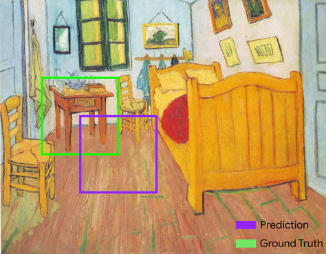
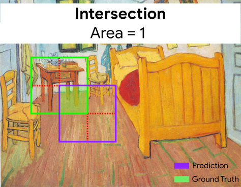
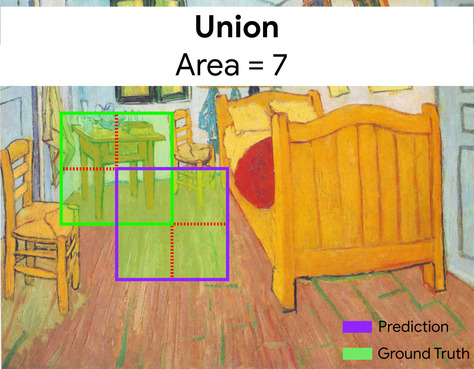
Here, the intersection of the bounding boxes for prediction and ground truth (below left) is 1, and the union of the bounding boxes for prediction and ground truth (below right) is 7, so the IoU is \(\frac{1}{7}\).

K

keypoints

#image

The coordinates of particular features in an image. For example, for an image recognition model that distinguishes flower species, keypoints might be the center of each petal, the stem, the stamen, and so on.

L

landmarks

#image

Synonym for keypoints.

M

MMIT

#language

#image

#generativeAI

Abbreviation for multimodal instruction-tuned.

MNIST

#image

A public-domain dataset compiled by LeCun, Cortes, and Burges containing 60,000 images, each image showing how a human manually wrote a particular digit from 0–9. Each image is stored as a 28x28 array of integers, where each integer is a grayscale value between 0 and 255, inclusive.

MNIST is a canonical dataset for machine learning, often used to test new machine learning approaches. For details, see The MNIST Database of Handwritten Digits.

MOE

#language

#image

#generativeAI

Abbreviation for mixture of experts.

P

pooling

#image

Reducing a matrix (or matrixes) created by an earlier convolutional layer to a smaller matrix. Pooling usually involves taking either the maximum or average value across the pooled area. For example, suppose we have the following 3x3 matrix:

A pooling operation, just like a convolutional operation, divides that matrix into slices and then slides that convolutional operation by strides. For example, suppose the pooling operation divides the convolutional matrix into 2x2 slices with a 1x1 stride. As the following diagram illustrates, four pooling operations take place. Imagine that each pooling operation picks the maximum value of the four in that slice:

Pooling helps enforce translational invariance in the input matrix.

Pooling for vision applications is known more formally as spatial pooling. Time-series applications usually refer to pooling as temporal pooling. Less formally, pooling is often called subsampling or downsampling.

post-trained model

#language

#image

#generativeAI

Loosely-defined term that typically refers to a pre-trained model that has gone through some post-processing, such as one or more of the following:

• Distillation
• Fine-tuning
• Instruction tuning

pre-trained model

#language

#image

#generativeAI

Typically, a model that has already been trained. The term could also mean a previously trained embedding vector.

The term pre-trained language model usually refers to an already trained large language model.

pre-training

#language

#image

#generativeAI

The initial training of a model on a large dataset. Some pre-trained models are clumsy giants and must typically be refined through additional training. For example, ML experts might pre-train a large language model on a vast text dataset, such as all the English pages in Wikipedia. Following pre-training, the resulting model might be further refined through any of the following techniques:

• distillation
• fine-tuning
• instruction tuning
• parameter-efficient tuning
• prompt-tuning

R

rotational invariance

#image

In an image classification problem, an algorithm's ability to successfully classify images even when the orientation of the image changes. For example, the algorithm can still identify a tennis racket whether it is pointing up, sideways, or down. Note that rotational invariance is not always desirable; for example, an upside-down 9 shouldn't be classified as a 9.

See also translational invariance and size invariance.

S

size invariance

#image

In an image classification problem, an algorithm's ability to successfully classify images even when the size of the image changes. For example, the algorithm can still identify a cat whether it consumes 2M pixels or 200K pixels. Note that even the best image classification algorithms still have practical limits on size invariance. For example, an algorithm (or human) is unlikely to correctly classify a cat image consuming only 20 pixels.

See also translational invariance and rotational invariance.

spatial pooling

#image

See pooling.

stride

#image

In a convolutional operation or pooling, the delta in each dimension of the next series of input slices. For example, the following animation demonstrates a (1,1) stride during a convolutional operation. Therefore, the next input slice starts one position to the right of the previous input slice. When the operation reaches the right edge, the next slice is all the way over to the left but one position down.

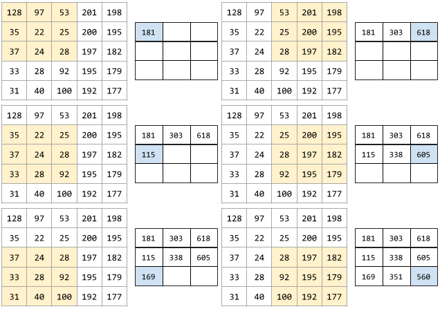
The preceding example demonstrates a two-dimensional stride. If the input matrix is three-dimensional, the stride would also be three-dimensional.

subsampling

#image

See pooling.

T

temperature

#language

#image

#generativeAI

A hyperparameter that controls the degree of randomness of a model's output. Higher temperatures result in more random output, while lower temperatures result in less random output.

Choosing the best temperature depends on the specific application and the preferred properties of the model's output. For example, you would probably raise the temperature when creating an application that generates creative output. Conversely, you would probably lower the temperature when building a model that classifies images or text in order to improve the model's accuracy and consistency.

Temperature is often used with softmax.

translational invariance

#image

In an image classification problem, an algorithm's ability to successfully classify images even when the position of objects within the image changes. For example, the algorithm can still identify a dog, whether it is in the center of the frame or at the left end of the frame.

See also size invariance and rotational invariance.