
您可以使用 Google 試算表 API 視需要在試算表中建立及更新圖表。本頁的範例說明如何使用 Sheets API 執行常見的圖表作業。
這些範例以 HTTP 要求的形式呈現,以便不受語言限制。如要瞭解如何使用 Google API 用戶端程式庫,以不同語言實作批次更新,請參閱「更新試算表」。
在這些範例中,預留位置 SPREADSHEET_ID 和 SHEET_ID 會指出您要提供這些 ID 的位置。你可以在試算表網址中找到試算表 ID。您可以使用 spreadsheets.get 方法取得工作表 ID。範圍使用 A1 標記法指定。範例範圍為 Sheet1!A1:D5。
此外,預留位置 CHART_ID 會指出特定圖表的 ID。您可以在使用 Sheets API 建立圖表時設定這個 ID,也可以讓 Sheets API 為您產生這個 ID。您可以使用 spreadsheets.get 方法取得現有圖表的 ID。
最後,預留位置 SOURCE_SHEET_ID 會指出含有來源資料的試算表。在這些範例中,這就是「圖表來源資料」下方列出的表格。
圖表來源資料
在這些範例中,假設所使用的試算表在第一個工作表 (「工作表 1」) 中含有下列來源資料。第一列中的字串是個別欄的標籤。如需從試算表中的其他工作表讀取資料的範例,請參閱「A1 符號」。
| A | B | C | D | E | |
| 1 | 型號 | 銷售 - 1 月 | 銷售 - 2 月 | 銷售 - 3 月 | 總銷售量 |
| 2 | D-01X | 68 | 74 | 60 | 202 |
| 3 | FR-0B1 | 97 | 76 | 88 | 261 |
| 4 | P-034 | 27 | 49 | 32 | 108 |
| 5 | P-105 | 46 | 44 | 67 | 157 |
| 6 | W-11 | 75 | 68 | 87 | 230 |
| 7 | W-24 | 74 | 52 | 62 | 188 |
新增柱狀圖
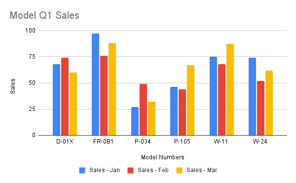
以下 spreadsheets.batchUpdate 程式碼範例說明如何使用 AddChartRequest 從來源資料建立並放置在新工作表中的資料欄圖表。這項要求會執行下列操作來設定圖表:
- 將圖表類型設為柱狀圖。
- 在圖表底部新增圖例。
- 設定圖表和軸標題。
- 設定 3 個資料列,代表 3 個不同月份的銷售量,並使用預設的格式和顏色。
要求通訊協定如下所示。
POST https://sheets.googleapis.com/v4/spreadsheets/SPREADSHEET_ID:batchUpdate
{
  "requests": [
    {
      "addChart": {
        "chart": {
          "spec": {
            "title": "Model Q1 Sales",
            "basicChart": {
              "chartType": "COLUMN",
              "legendPosition": "BOTTOM_LEGEND",
              "axis": [
                {
                  "position": "BOTTOM_AXIS",
                  "title": "Model Numbers"
                },
                {
                  "position": "LEFT_AXIS",
                  "title": "Sales"
                }
              ],
              "domains": [
                {
                  "domain": {
                    "sourceRange": {
                      "sources": [
                        {
                          "sheetId": SOURCE_SHEET_ID,
                          "startRowIndex": 0,
                          "endRowIndex": 7,
                          "startColumnIndex": 0,
                          "endColumnIndex": 1
                        }
                      ]
                    }
                  }
                }
              ],
              "series": [
                {
                  "series": {
                    "sourceRange": {
                      "sources": [
                        {
                          "sheetId": SOURCE_SHEET_ID,
                          "startRowIndex": 0,
                          "endRowIndex": 7,
                          "startColumnIndex": 1,
                          "endColumnIndex": 2
                        }
                      ]
                    }
                  },
                  "targetAxis": "LEFT_AXIS"
                },
                {
                  "series": {
                    "sourceRange": {
                      "sources": [
                        {
                          "sheetId": SOURCE_SHEET_ID,
                          "startRowIndex": 0,
                          "endRowIndex": 7,
                          "startColumnIndex": 2,
                          "endColumnIndex": 3
                        }
                      ]
                    }
                  },
                  "targetAxis": "LEFT_AXIS"
                },
                {
                  "series": {
                    "sourceRange": {
                      "sources": [
                        {
                          "sheetId": SOURCE_SHEET_ID,
                          "startRowIndex": 0,
                          "endRowIndex": 7,
                          "startColumnIndex": 3,
                          "endColumnIndex": 4
                        }
                      ]
                    }
                  },
                  "targetAxis": "LEFT_AXIS"
                }
              ],
              "headerCount": 1
            }
          },
          "position": {
            "newSheet": true
          }
        }
      }
    }
  ]
}
這項要求會在新工作表中建立圖表,如下所示:
新增圓餅圖
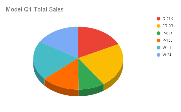
以下 spreadsheets.batchUpdate 程式碼範例說明如何使用 AddChartRequest 從來源資料建立 3D 圓餅圖。這項要求會執行下列操作來設定圖表:
- 設定圖表標題。
- 在圖表右側新增圖例。
- 將圖表設為 3D 圓餅圖。請注意,3D 圓餅圖無法像平面圓餅圖一樣,在圓心處顯示「圓環洞」。
- 將圖表資料序列設為每個型號的總銷售量。
- 將圖表固定在 SHEET_ID 指定工作表的 C3 儲存格上,並在 X 和 Y 方向上偏移 50 個像素。
要求通訊協定如下所示。
POST https://sheets.googleapis.com/v4/spreadsheets/SPREADSHEET_ID:batchUpdate
{
  "requests": [
    {
      "addChart": {
        "chart": {
          "spec": {
            "title": "Model Q1 Total Sales",
            "pieChart": {
              "legendPosition": "RIGHT_LEGEND",
              "threeDimensional": true,
              "domain": {
                "sourceRange": {
                  "sources": [
                    {
                      "sheetId": SOURCE_SHEET_ID,
                      "startRowIndex": 0,
                      "endRowIndex": 7,
                      "startColumnIndex": 0,
                      "endColumnIndex": 1
                    }
                  ]
                }
              },
              "series": {
                "sourceRange": {
                  "sources": [
                    {
                      "sheetId": SOURCE_SHEET_ID,
                      "startRowIndex": 0,
                      "endRowIndex": 7,
                      "startColumnIndex": 4,
                      "endColumnIndex": 5
                    }
                  ]
                }
              },
            }
          },
          "position": {
            "overlayPosition": {
              "anchorCell": {
                "sheetId": SHEET_ID,
                "rowIndex": 2,
                "columnIndex": 2
              },
              "offsetXPixels": 50,
              "offsetYPixels": 50
            }
          }
        }
      }
    }
  ]
}
這項要求會建立如下圖所示的圖表:
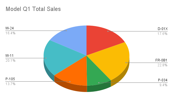
或者,您也可以在要求中將 legendPosition 值從 RIGHT_LEGEND 更新為 LABELED_LEGEND,以便將圖例值連結至圓餅圖切片。
'legendPosition': 'LABELED_LEGEND',
更新後的要求會建立如下圖所示的圖表:
使用多個非相鄰範圍新增折線圖
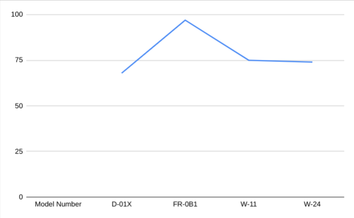
以下 spreadsheets.batchUpdate 程式碼範例說明如何使用 AddChartRequest 從來源資料建立折線圖,並將其放在來源工作表中。選取不連續的範圍,可用於從 ChartSourceRange 中排除資料列。
這項要求會執行下列操作來設定圖表:
- 將圖表類型設為折線圖。
- 設定水平 X 軸標題。
- 設定代表銷售的資料序列。它會將 A1:A3 和 A6:A7 設為
domain,將 B1:B3 和 B6:B7 設為series,並使用預設的格式和顏色。範圍會在要求網址中使用 A1 符號指定。 - 將圖表固定在 SHEET_ID 指定試算表的 H8 儲存格上。
要求通訊協定如下所示。
POST https://sheets.googleapis.com/v4/spreadsheets/SPREADSHEET_ID:batchUpdate
{
  "requests": [
    {
      "addChart": {
        "chart": {
          "spec": {
            "basicChart": {
              "chartType": "LINE",
              "domains": [
                {
                  "domain": {
                    "sourceRange": {
                      "sources": [
                        {
                          "startRowIndex": 0,
                          "endRowIndex": 3,
                          "startColumnIndex": 0,
                          "endColumnIndex": 1,
                          "sheetId": SOURCE_SHEET_ID
                        },
                        {
                          "startRowIndex": 5,
                          "endRowIndex": 7,
                          "startColumnIndex": 0,
                          "endColumnIndex": 1,
                          "sheetId": SOURCE_SHEET_ID
                        }
                      ]
                    }
                  }
                }
              ],
              "series": [
                {
                  "series": {
                    "sourceRange": {
                      "sources": [
                        {
                          "startRowIndex": 0,
                          "endRowIndex": 3,
                          "startColumnIndex": 1,
                          "endColumnIndex": 2,
                          "sheetId": SOURCE_SHEET_ID
                        },
                        {
                          "startRowIndex": 5,
                          "endRowIndex": 7,
                          "startColumnIndex": 1,
                          "endColumnIndex": 2,
                          "sheetId": SOURCE_SHEET_ID
                        }
                      ]
                    }
                  }
                }
              ]
            }
          },
          "position": {
            "overlayPosition": {
              "anchorCell": {
                "sheetId": SOURCE_SHEET_ID,
                "rowIndex": 8,
                "columnIndex": 8
              }
            }
          }
        }
      }
    }
  ]
}
這項要求會在新工作表中建立圖表,如下所示:
刪除圖表
以下 spreadsheets.batchUpdate 程式碼範例說明如何使用 DeleteEmbeddedObjectRequest 刪除 CHART_ID 指定的圖表。
要求通訊協定如下所示。
POST https://sheets.googleapis.com/v4/spreadsheets/SPREADSHEET_ID:batchUpdate
{
  "requests": [
    {
      "deleteEmbeddedObject": {
        "objectId": CHART_ID
      }
    }
  ]
}
編輯圖表的屬性
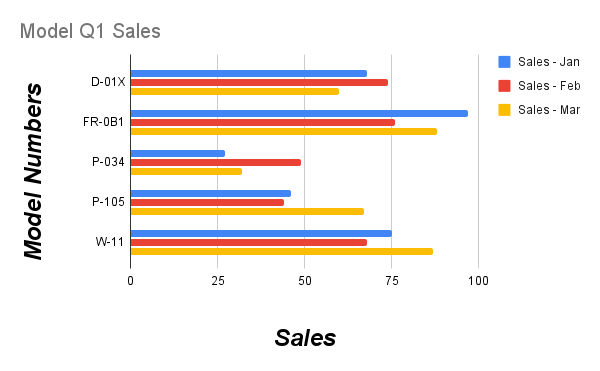
以下 spreadsheets.batchUpdate 程式碼範例說明如何使用 UpdateChartSpecRequest 編輯在「新增資料欄圖表」食譜中建立的圖表,修改圖表的資料、類型和外觀。您無法個別變更圖表屬性子集。如要進行編輯,您必須使用 UpdateChartSpecRequest 提供整個 spec 欄位。基本上,編輯圖表規格時,必須將其替換為新的規格。
以下要求會更新原始圖表 (由 CHART_ID 指定):
- 將圖表類型設為
BAR。 - 將圖例移至圖表右側。
- 反轉軸,讓「Sales」位於底部軸,「Model Numbers」位於左側軸。
- 將軸標題格式設為 24 點字型、粗體和斜體。
- 從圖表中移除「W-24」資料 (圖表來源資料中的第 7 列)。
要求通訊協定如下所示。
POST https://sheets.googleapis.com/v4/spreadsheets/SPREADSHEET_ID:batchUpdate
{
  "requests": [
    {
      "updateChartSpec": {
        "chartId": CHART_ID,
        "spec": {
          "title": "Model Q1 Sales",
          "basicChart": {
            "chartType": "BAR",
            "legendPosition": "RIGHT_LEGEND",
            "axis": [
              {
                "format": {
                  "bold": true,
                  "italic": true,
                  "fontSize": 24
                },
                "position": "BOTTOM_AXIS",
                "title": "Sales"
              },
              {
                "format": {
                  "bold": true,
                  "italic": true,
                  "fontSize": 24
                },
                "position": "LEFT_AXIS",
                "title": "Model Numbers"
              }
            ],
            "domains": [
              {
                "domain": {
                  "sourceRange": {
                    "sources": [
                      {
                        "sheetId": SOURCE_SHEET_ID,
                        "startRowIndex": 0,
                        "endRowIndex": 6,
                        "startColumnIndex": 0,
                        "endColumnIndex": 1
                      }
                    ]
                  }
                }
              }
            ],
            "series": [
              {
                "series": {
                  "sourceRange": {
                    "sources": [
                      {
                        "sheetId": SOURCE_SHEET_ID,
                        "startRowIndex": 0,
                        "endRowIndex": 6,
                        "startColumnIndex": 1,
                        "endColumnIndex": 2
                      }
                    ]
                  }
                },
                "targetAxis": "BOTTOM_AXIS"
              },
              {
                "series": {
                  "sourceRange": {
                    "sources": [
                      {
                        "sheetId": SOURCE_SHEET_ID,
                        "startRowIndex": 0,
                        "endRowIndex": 6,
                        "startColumnIndex": 2,
                        "endColumnIndex": 3
                      }
                    ]
                  }
                },
                "targetAxis": "BOTTOM_AXIS"
              },
              {
                "series": {
                  "sourceRange": {
                    "sources": [
                      {
                        "sheetId": SOURCE_SHEET_ID,
                        "startRowIndex": 0,
                        "endRowIndex": 6,
                        "startColumnIndex": 3,
                        "endColumnIndex": 4
                      }
                    ]
                  }
                },
                "targetAxis": "BOTTOM_AXIS"
              }
            ],
            "headerCount": 1
          }
        }
      }
    }
  ]
}
提出要求後,圖表會顯示如下:
移動或調整圖表大小
以下 spreadsheets.batchUpdate 程式碼範例說明如何使用 UpdateEmbeddedObjectPositionRequest 移動及調整圖表大小。提出要求後,CHART_ID 指定的圖表如下:
- 錨定於原始工作表的 A5 儲存格。
- 在 X 方向偏移 100 個像素。
- 將圖表尺寸調整為 1200 x 742 像素 (圖表的預設大小為 600 x 371 像素)。
這項要求只會變更使用 fields 參數指定的屬性。其他屬性 (例如 offsetYPixels) 則會保留原始值。
要求通訊協定如下所示。
POST https://sheets.googleapis.com/v4/spreadsheets/SPREADSHEET_ID:batchUpdate
{
  "requests": [
    {
      "updateEmbeddedObjectPosition": {
        "objectId": CHART_ID,
        "newPosition": {
          "overlayPosition": {
            "anchorCell": {
              "rowIndex": 4,
              "columnIndex": 0
            },
            "offsetXPixels": 100,
            "widthPixels": 1200,
            "heightPixels": 742
          }
        },
        "fields": "anchorCell(rowIndex,columnIndex),offsetXPixels,widthPixels,heightPixels"
      }
    }
  ]
}
讀取圖表資料
以下 spreadsheets.get 程式碼範例說明如何從試算表取得圖表資料。fields 查詢參數指定只傳回圖表資料。
這個方法呼叫的回應是 spreadsheet 物件,其中包含 sheet 物件的陣列。工作表中的所有圖表都會在 sheet 物件中顯示。如果回應欄位設為預設值,則會從回應中省略。
在本範例中,第一個工作表 (SOURCE_SHEET_ID) 沒有任何圖表,因此會傳回一對空格中括號。第二個工作表包含「新增柱狀圖」所建立的圖表,其他內容則沒有。
要求通訊協定如下所示。
GET https://sheets.googleapis.com/v4/spreadsheets/SPREADSHEET_ID?fields=sheets(charts)
{
  "sheets": [
    {},
    {
      "charts": [
        {
          "chartId": CHART_ID,
          "position": {
            "sheetId": SHEET_ID
          },
          "spec": {
            "basicChart": {
              "axis": [
                {
                  "format": {
                    "bold": false,
                    "italic": false
                  },
                  "position": "BOTTOM_AXIS",
                  "title": "Model Numbers"
                },
                {
                  "format": {
                    "bold": false,
                    "italic": false
                  },
                  "position": "LEFT_AXIS",
                  "title": "Sales"
                }
              ],
              "chartType": "COLUMN",
              "domains": [
                {
                  "domain": {
                    "sourceRange": {
                      "sources": [
                        {
                          "endColumnIndex": 1
                          "endRowIndex": 7,
                          "sheetId": SOURCE_SHEET_ID,
                          "startColumnIndex": 0,
                          "startRowIndex": 0,
                        }
                      ]
                    }
                  }
                }
              ],
              "legendPosition": "BOTTOM_LEGEND",
              "series": [
                {
                  "series": {
                    "sourceRange": {
                      "sources": [
                        {
                          "endColumnIndex": 2,
                          "endRowIndex": 7,
                          "sheetId": SOURCE_SHEET_ID,
                          "startColumnIndex": 1,
                          "startRowIndex": 0,
                        }
                      ]
                    }
                  },
                  "targetAxis": "LEFT_AXIS"
                },
                {
                  "series": {
                    "sourceRange": {
                      "sources": [
                        {
                          "endColumnIndex": 3,
                          "endRowIndex": 7,
                          "sheetId": SOURCE_SHEET_ID,
                          "startColumnIndex": 2,
                          "startRowIndex": 0,
                        }
                      ]
                    }
                  },
                  "targetAxis": "LEFT_AXIS"
                },
                {
                  "series": {
                    "sourceRange": {
                      "sources": [
                        {
                          "endColumnIndex": 4,
                          "endRowIndex": 7,
                          "sheetId": SOURCE_SHEET_ID,
                          "startColumnIndex": 3,
                          "startRowIndex": 0,
                        }
                      ]
                    }
                  },
                  "targetAxis": "LEFT_AXIS"
                }
              ]
            },
            "hiddenDimensionStrategy": "SKIP_HIDDEN_ROWS_AND_COLUMNS",
            "title": "Model Q1 Sales",
          },
        }
      ]
    }
  ]
}