このセクションでは、Google Cloud の
モデルです。手順 3 では、
S/W 比率を使用して、N グラム モデルまたはシーケンス モデルの使用を選択しました。
それでは、分類アルゴリズムを記述してトレーニングしましょう。使用するのは
TensorFlow:
tf.keras
API を使用します
Keras での ML モデルの構築は、すべてを組み合わせることが重要 レイヤ、データ処理構成要素です。 ブロックします。これらのレイヤにより、必要な変換のシーケンスを モデルのことです。この学習アルゴリズムは単一のテキスト入力と レイヤの線形スタックを作成できます。 使用 シーケンシャル モデル API
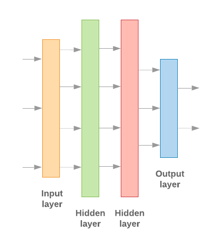
図 9: レイヤの線形スタック
入力レイヤと中間レイヤの構成は異なります。 N グラムとシーケンス モデルのどちらを使用するかによって異なります。しかし、 モデルタイプに関係なく、特定の問題の最後のレイヤは同じになります。
最後のレイヤを作成する
クラスが 2 つ(バイナリ分類)しかない場合、モデルは
計算します。たとえば、特定の入力サンプルに対して 0.2 を出力する
「このサンプルがファースト クラス(クラス 1)にある確率が 20%、クラス 1 である確率が 80% である」という意味です。
「クラス 0」です。このような確率スコアを出力するには、
活性化関数
最後のレイヤは、
シグモイド関数
および
損失関数
使用するのは、入力シーケンスの
バイナリ交差エントロピー。
(左の図 10 を参照)。
3 つ以上のクラス(マルチクラス分類)がある場合、このモデルは
クラスごとに 1 つの確率スコアが出力されます。これらのスコアの合計は
1.たとえば、{0: 0.2, 1: 0.7, 2: 0.1} を出力すると、「その信頼度が 20% である」という意味になります。
このサンプルはクラス 0 にあり、70% がクラス 1、10% がクラス 1 にあります。
クラス 2」を選択します。これらのスコアを出力するために、最後のレイヤの活性化関数
ソフトマックスとし、モデルのトレーニングに使用する損失関数は
カテゴリ交差エントロピーです(右の図 10 をご覧ください)。
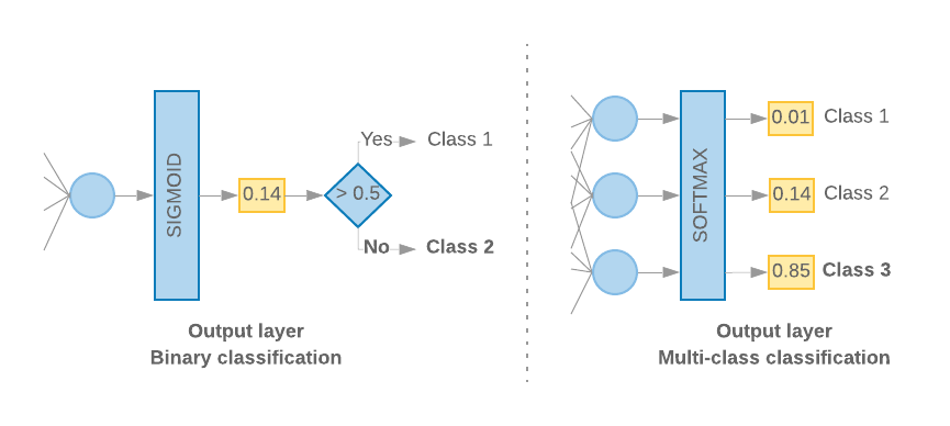
図 10: 最後のレイヤ
次のコードは、クラスの数を入力として受け取る関数を定義しています。 適切な数のレイヤユニット(バイナリの場合は 1 ユニット)を出力します。 分類するそれ以外の場合はクラスごとに 1 ユニット)と適切なアクティベーション 関数:
def _get_last_layer_units_and_activation(num_classes):
    """Gets the # units and activation function for the last network layer.

    # Arguments
        num_classes: int, number of classes.

    # Returns
        units, activation values.
    """
    if num_classes == 2:
        activation = 'sigmoid'
        units = 1
    else:
        activation = 'softmax'
        units = num_classes
    return units, activation
次の 2 つのセクションでは、残りのモデルの作成について説明します。 N グラム モデルとシーケンス モデル用のレイヤです。
S/W の比率が小さいほど、N グラムモデルの方がパフォーマンスが向上することがわかっています。
Sequence-to-Sequenceシーケンス モデルは、シーケンスの
ベクトルが生成されます。これは、エンベディング関係が最初のレイヤで学習され、
これは多数のサンプルで最もよく実現します。
N グラム モデルの構築 [オプション A]
トークンを独立して処理するモデルを指します( を N グラムモデルとして表現します。シンプルな多層パーセプトロン( ロジスティック回帰 勾配ブースティングマシン およびサポート ベクトル マシンモデル) すべてこのカテゴリに分類されます。使用できず、 並べ替えられます。
前述の N グラムモデルのいくつかの性能を比較しました。 より多層パーセプトロン(MLP)の方が一般的に その他のオプションですMLP は定義と理解が簡単で、精度が高く、 比較的少ない計算量で実行できます。
次のコードは、tf.keras で 2 層の MLP モデルを定義します。 正則化用のドロップアウト レイヤ 予防的に 過学習 生成します。
from tensorflow.python.keras import models
from tensorflow.python.keras.layers import Dense
from tensorflow.python.keras.layers import Dropout

def mlp_model(layers, units, dropout_rate, input_shape, num_classes):
    """Creates an instance of a multi-layer perceptron model.

    # Arguments
        layers: int, number of `Dense` layers in the model.
        units: int, output dimension of the layers.
        dropout_rate: float, percentage of input to drop at Dropout layers.
        input_shape: tuple, shape of input to the model.
        num_classes: int, number of output classes.

    # Returns
        An MLP model instance.
    """
    op_units, op_activation = _get_last_layer_units_and_activation(num_classes)
    model = models.Sequential()
    model.add(Dropout(rate=dropout_rate, input_shape=input_shape))

    for _ in range(layers-1):
        model.add(Dense(units=units, activation='relu'))
        model.add(Dropout(rate=dropout_rate))

    model.add(Dense(units=op_units, activation=op_activation))
    return model
シーケンス モデルの構築 [オプション B]
トークンの近接性から学習できるモデルをシーケンス 構築できますこれには、CNN および RNN クラスのモデルが含まれます。データは ベクトルが生成されます。
シーケンス モデルは通常、学習するパラメータをより大量に持ちます。最初の エンべディング レイヤです。エンべディング レイヤでは、 密ベクトル空間での単語間の結合を意味します。単語の関係性を学ぶことは効果的 最も良い結果を出力できます
特定のデータセット内の単語は、多くの場合、そのデータセットに固有のものではありません。このように 他のデータセットを使用して、データセット内の単語間の関係を学習する。 そのためには、別のデータセットから学習したエンべディングを Embedding レイヤです。これらのエンベディングは、事前トレーニング済み Embeddings です。事前トレーニング済みのエンべディングを使用すると、 学習プロセスに集中できます。
大規模言語モデルを使用してトレーニングされた事前トレーニング済みエンベディングを使用できます。 GloVe などのコーパス。GloVe は 複数のコーパス(主に Wikipedia)でトレーニングされています。Google の GloVe エンべディングのバージョンを使用してシーケンスモデルを 事前トレーニング済みのエンベディングの重みを固定して、 モデルのパフォーマンスは良好ではありませんでした。その理由は、データのコンテキストが エンべディング レイヤのトレーニング データの内容がコンテキスト 確認しました
Wikipedia のデータでトレーニングされた GloVe のエンベディングは、言語と一致しない場合がある パターンを検出しました。推定される関係には、ある程度の つまり、エンベディングの重みにコンテキスト チューニングが必要になる場合があります。これには、 2 つのステージがあります。
最初の実行では、エンベディング レイヤの重みを固定して、残りを 学習します。この実行が終了すると、モデルの重みが状態に到達します。 初期化されていない値よりもはるかに優れています。2 回目の実行では、 エンベディング レイヤも学習できるようにして、すべての重みを微調整する ファイアウォールルールがありますこのプロセスをファインチューニングされたエンベディングの使用と呼びます。
エンベディングをファインチューニングすると精度が向上します。ただし、これは ネットワークのトレーニングに必要な演算能力の増加に 費用がかかります与えられた 十分な数のサンプルが用意されていれば、エンベディング 構築します。
S/W > 15Kについては、ゼロから効果的に開始したことが確認されています。 ファインチューニングされたエンベディングを使用した場合とほぼ同じ精度が得られます。
CNN、sepCNN、 RNN(LSTM &GRU)、CNN-RNN、スタック RNN(スタックされた RNN を 構築できます畳み込みネットワーク亜種である sepCNN が、 多くの場合、データ効率とコンピューティング効率に優れ、 サポートしています。
<ph type="x-smartling-placeholder">次のコードは、4 レイヤの sepCNN モデルを構築します。
from tensorflow.python.keras import models
from tensorflow.python.keras import initializers
from tensorflow.python.keras import regularizers

from tensorflow.python.keras.layers import Dense
from tensorflow.python.keras.layers import Dropout
from tensorflow.python.keras.layers import Embedding
from tensorflow.python.keras.layers import SeparableConv1D
from tensorflow.python.keras.layers import MaxPooling1D
from tensorflow.python.keras.layers import GlobalAveragePooling1D

def sepcnn_model(blocks,
                 filters,
                 kernel_size,
                 embedding_dim,
                 dropout_rate,
                 pool_size,
                 input_shape,
                 num_classes,
                 num_features,
                 use_pretrained_embedding=False,
                 is_embedding_trainable=False,
                 embedding_matrix=None):
    """Creates an instance of a separable CNN model.

    # Arguments
        blocks: int, number of pairs of sepCNN and pooling blocks in the model.
        filters: int, output dimension of the layers.
        kernel_size: int, length of the convolution window.
        embedding_dim: int, dimension of the embedding vectors.
        dropout_rate: float, percentage of input to drop at Dropout layers.
        pool_size: int, factor by which to downscale input at MaxPooling layer.
        input_shape: tuple, shape of input to the model.
        num_classes: int, number of output classes.
        num_features: int, number of words (embedding input dimension).
        use_pretrained_embedding: bool, true if pre-trained embedding is on.
        is_embedding_trainable: bool, true if embedding layer is trainable.
        embedding_matrix: dict, dictionary with embedding coefficients.

    # Returns
        A sepCNN model instance.
    """
    op_units, op_activation = _get_last_layer_units_and_activation(num_classes)
    model = models.Sequential()

    # Add embedding layer. If pre-trained embedding is used add weights to the
    # embeddings layer and set trainable to input is_embedding_trainable flag.
    if use_pretrained_embedding:
        model.add(Embedding(input_dim=num_features,
                            output_dim=embedding_dim,
                            input_length=input_shape[0],
                            weights=[embedding_matrix],
                            trainable=is_embedding_trainable))
    else:
        model.add(Embedding(input_dim=num_features,
                            output_dim=embedding_dim,
                            input_length=input_shape[0]))

    for _ in range(blocks-1):
        model.add(Dropout(rate=dropout_rate))
        model.add(SeparableConv1D(filters=filters,
                                  kernel_size=kernel_size,
                                  activation='relu',
                                  bias_initializer='random_uniform',
                                  depthwise_initializer='random_uniform',
                                  padding='same'))
        model.add(MaxPooling1D(pool_size=pool_size))

    model.add(SeparableConv1D(filters=filters * 2,
                              kernel_size=kernel_size,
                              activation='relu',
                              bias_initializer='random_uniform',
                              depthwise_initializer='random_uniform',
                              padding='same'))
    model.add(GlobalAveragePooling1D())
    model.add(Dropout(rate=dropout_rate))
    model.add(Dense(op_units, activation=op_activation))
    return model
モデルのトレーニング
モデル アーキテクチャを構築したので、モデルをトレーニングする必要があります。 トレーニングでは、モデルの現在の状態に基づいて予測を行います。 予測の誤りの程度の計算、重みまたは予測の 使用してモデルの誤差を最小化し、モデルの 向上しますモデルが収束し 学びます。このプロセスでは主に 3 つのパラメータを選択します(表を参照) 2.)
- 指標: 指標。accuracy を使用した 使用しています
- 損失関数: 損失値を計算するために使用される関数 トレーニング プロセスで、モデルのパフォーマンスを調整し、 ネットワークの重み分類問題には、交差エントロピー損失が適しています。
- オプティマイザー: ネットワークの重みを決定する関数 損失関数の出力に基づいて更新されます。広く使われている Adam オプティマイザーを Google のテストで使用する。
Keras では、Keras アプリケーションの コンパイル メソッドを呼び出します。
表 2: 学習パラメータ
| 学習パラメータ | 値 |
|---|---|
| 指標 | accuracy |
| 損失関数 - バイナリ分類 | binary_crossentropy |
| 損失関数 - マルチクラス分類 | sparse_categorical_crossentropy |
| オプティマイザー | Adam |
実際のトレーニングは、
fit メソッドを使用します。
広告ユニットのサイズや
この方法では、ほとんどのコンピューティング サイクルが消費されます。各
トレーニングの反復処理、batch_size トレーニング データからのサンプル数
を使用して損失を計算し、この値に基づいて重みを一度更新します。
モデルがデータ全体を認識すると、トレーニング プロセスは epoch を
トレーニングデータセットです各エポックの終了時に、検証用データセットを使用して
モデルの学習状況を評価できますデータセットを使ってトレーニングを
所定のエポック数で繰り返し実行されることです。早期に停止することで最適化でき
連続するエポック間で検証精度が安定した場合、
モデルのトレーニングが行われなくなります
| ハイパーパラメータのトレーニング | 値 |
|---|---|
| 学習率 | 1 ~ 3 |
| エポック | 1000 |
| バッチサイズ | 512 |
| 早期停止 | パラメータ: Val_loss, latency: 1 |
表 3: ハイパーパラメータのトレーニング
次の Keras コードでは、パラメータを使用してトレーニング プロセスを実装しています 表 2 と上記 3:
def train_ngram_model(data,
                      learning_rate=1e-3,
                      epochs=1000,
                      batch_size=128,
                      layers=2,
                      units=64,
                      dropout_rate=0.2):
    """Trains n-gram model on the given dataset.

    # Arguments
        data: tuples of training and test texts and labels.
        learning_rate: float, learning rate for training model.
        epochs: int, number of epochs.
        batch_size: int, number of samples per batch.
        layers: int, number of `Dense` layers in the model.
        units: int, output dimension of Dense layers in the model.
        dropout_rate: float: percentage of input to drop at Dropout layers.

    # Raises
        ValueError: If validation data has label values which were not seen
            in the training data.
    """
    # Get the data.
    (train_texts, train_labels), (val_texts, val_labels) = data

    # Verify that validation labels are in the same range as training labels.
    num_classes = explore_data.get_num_classes(train_labels)
    unexpected_labels = [v for v in val_labels if v not in range(num_classes)]
    if len(unexpected_labels):
        raise ValueError('Unexpected label values found in the validation set:'
                         ' {unexpected_labels}. Please make sure that the '
                         'labels in the validation set are in the same range '
                         'as training labels.'.format(
                             unexpected_labels=unexpected_labels))

    # Vectorize texts.
    x_train, x_val = vectorize_data.ngram_vectorize(
        train_texts, train_labels, val_texts)

    # Create model instance.
    model = build_model.mlp_model(layers=layers,
                                  units=units,
                                  dropout_rate=dropout_rate,
                                  input_shape=x_train.shape[1:],
                                  num_classes=num_classes)

    # Compile model with learning parameters.
    if num_classes == 2:
        loss = 'binary_crossentropy'
    else:
        loss = 'sparse_categorical_crossentropy'
    optimizer = tf.keras.optimizers.Adam(lr=learning_rate)
    model.compile(optimizer=optimizer, loss=loss, metrics=['acc'])

    # Create callback for early stopping on validation loss. If the loss does
    # not decrease in two consecutive tries, stop training.
    callbacks = [tf.keras.callbacks.EarlyStopping(
        monitor='val_loss', patience=2)]

    # Train and validate model.
    history = model.fit(
            x_train,
            train_labels,
            epochs=epochs,
            callbacks=callbacks,
            validation_data=(x_val, val_labels),
            verbose=2,  # Logs once per epoch.
            batch_size=batch_size)

    # Print results.
    history = history.history
    print('Validation accuracy: {acc}, loss: {loss}'.format(
            acc=history['val_acc'][-1], loss=history['val_loss'][-1]))

    # Save model.
    model.save('IMDb_mlp_model.h5')
    return history['val_acc'][-1], history['val_loss'][-1]
シーケンス モデルをトレーニングするためのコード例については、こちらをご覧ください。