이 섹션에서는
있습니다. 3단계에서는
S/W 비율을 사용하여 N-그램 모델 또는 시퀀스 모델을 사용하기로 선택했습니다.
이제 분류 알고리즘을 작성하고 학습시킬 차례입니다. 여기서는
TensorFlow
tf.keras
API를 제공합니다
Keras를 사용한 머신러닝 모델 빌드의 모든 것 데이터 처리 빌딩 블록, 즉 레고를 조립할 때와 마찬가지로 있습니다. 이러한 레이어를 사용하면 원하는 변환 시퀀스를 모델을 학습시키는 작업도 반복해야 합니다 학습 알고리즘이 단일 텍스트 입력을 받아들일 때 단일 분류를 출력하려면 선형 레이어 스택을 만들어 사용 순차적 모델 API에 액세스할 수 있습니다.
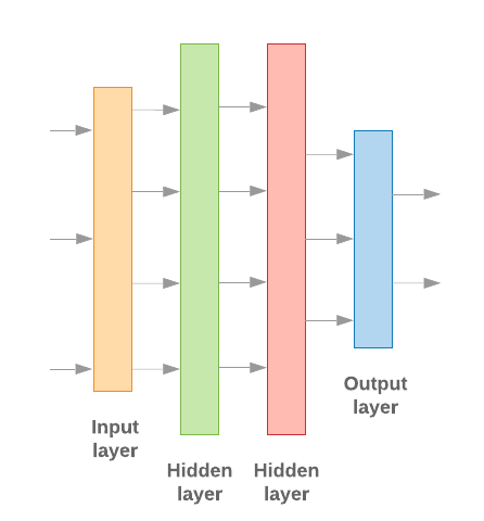
그림 9: 선형 레이어 스택
입력 레이어와 중간 레이어는 서로 다르게 구성됩니다. 또는 시퀀스 모델 중 어느 것을 빌드하는지에 따라 다릅니다. 하지만 마지막 레이어는 주어진 문제에 대해 동일합니다.
마지막 레이어 생성
클래스가 2개만 있는 경우 (이진 분류) 모델은
단일 확률 점수입니다. 예를 들어 지정된 입력 샘플에 대해 0.2를 출력합니다.
'이 표본이 첫 번째 클래스(클래스 1)에 해당한다는 신뢰도 20%, 첫 번째 클래스(클래스 1)'에
두 번째 클래스 (클래스 0)에 있습니다.” 이러한 확률 점수를 출력하려면
활성화 함수
마지막 레이어의 최상위 레이어는
시그모이드 함수,
및
손실 함수
모델이 학습하는 데 사용되는
바이너리 교차 엔트로피.
왼쪽의 그림 10을 참고하세요.
클래스가 3개 이상 있는 경우 (다중 클래스 분류)
클래스당 하나의 확률 점수를 출력해야 합니다. 이 점수의 합은
1. 예를 들어, {0: 0.2, 1: 0.7, 2: 0.1} 출력은
이 샘플은 클래스 0에 있고 클래스 1에 있는 70%, 클래스 1에 있는 10% 입니다.
수업 2." 이러한 점수를 출력하기 위해 마지막 레이어의 활성화 함수는
소프트맥스여야 하고 모델 학습에 사용되는 손실 함수는
교차 엔트로피를 생성합니다. 오른쪽 그림 10을 참고하세요.
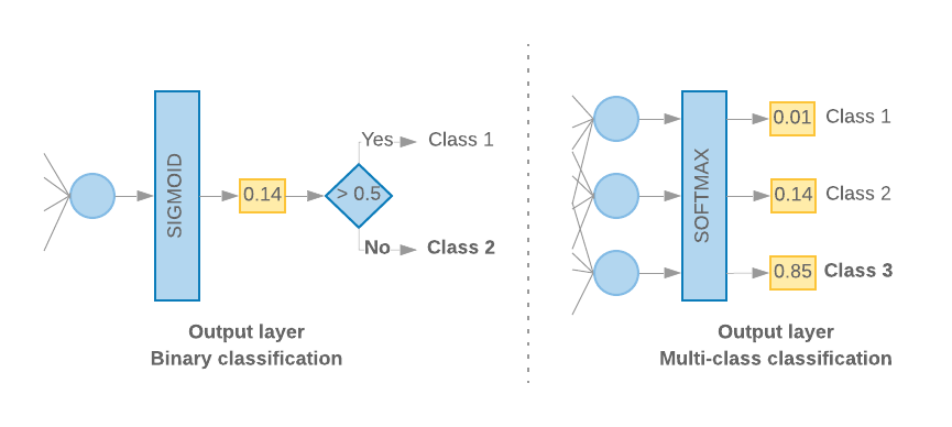
그림 10: 마지막 레이어
다음 코드는 클래스 수를 입력으로 사용하는 함수를 정의합니다. 적절한 수의 레이어 단위 (2진수의 경우 1단위)를 분류 적절한 활성화를 사용해야 합니다. 함수:
def _get_last_layer_units_and_activation(num_classes):
    """Gets the # units and activation function for the last network layer.

    # Arguments
        num_classes: int, number of classes.

    # Returns
        units, activation values.
    """
    if num_classes == 2:
        activation = 'sigmoid'
        units = 1
    else:
        activation = 'softmax'
        units = num_classes
    return units, activation
다음 두 섹션에서는 나머지 모델을 만드는 방법을 안내합니다. 뉴그램 계층에 대해 배웠습니다.
S/W 비율이 작으면 N-그램 모델이 더 나은 성능을 보임
더 높습니다. 시퀀스 모델은
벡터로 변환합니다. 이는 임베딩 관계는
많은 샘플에 대해 가장 잘 작동합니다.
N-그램 모델 빌드[옵션 A]
토큰을 독립적으로 처리하는 모델이라고 합니다( 계정 워드 순서)를 N-그램 모델로 변환합니다. 단순 멀티 레이어 퍼셉트론( 로지스틱 회귀 경사 부스팅 머신, 벡터 머신 모델 지원). 모두 이 카테고리에 속합니다. 그들은 그 어떤 정보도 사용할 수 있습니다.
위에서 언급한 일부 N-그램 모델의 성능을 비교했으며, 다중 레이어 퍼셉트론 (MLP)이 일반적으로 MLP의 성능보다 확인할 수 있습니다 MLP는 정의 및 이해하기 쉽고, 높은 정확성을 제공하며, 상대적으로 적은 계산이 필요합니다
다음 코드는 tf.keras의 두 레이어 MLP 모델을 정의하고 정규화를 위한 드롭아웃 레이어 방어하기 위해 과적합 학습 샘플로 보냅니다
from tensorflow.python.keras import models
from tensorflow.python.keras.layers import Dense
from tensorflow.python.keras.layers import Dropout

def mlp_model(layers, units, dropout_rate, input_shape, num_classes):
    """Creates an instance of a multi-layer perceptron model.

    # Arguments
        layers: int, number of `Dense` layers in the model.
        units: int, output dimension of the layers.
        dropout_rate: float, percentage of input to drop at Dropout layers.
        input_shape: tuple, shape of input to the model.
        num_classes: int, number of output classes.

    # Returns
        An MLP model instance.
    """
    op_units, op_activation = _get_last_layer_units_and_activation(num_classes)
    model = models.Sequential()
    model.add(Dropout(rate=dropout_rate, input_shape=input_shape))

    for _ in range(layers-1):
        model.add(Dense(units=units, activation='relu'))
        model.add(Dropout(rate=dropout_rate))

    model.add(Dense(units=op_units, activation=op_activation))
    return model
시퀀스 모델 빌드[옵션 B]
토큰의 인접성을 통해 학습할 수 있는 모델을 시퀀스라고 지칭합니다. 모델을 학습시키는 작업도 반복해야 합니다 여기에는 모델의 CNN 및 RNN 클래스가 포함됩니다. 데이터는 다음과 같이 전처리됩니다. 시퀀스 벡터로 변환합니다.
시퀀스 모델은 일반적으로 학습해야 할 매개변수 수가 더 많습니다. 첫 번째 모델의 관계를 학습하는 임베딩 레이어가 있습니다. 단어 사이에 배치하기 때문입니다. 단어 관계 학습 여러 샘플에 비해 가장 우수한 성능을 보여줍니다.
특정 데이터 세트의 단어는 해당 데이터 세트에 고유하지 않을 가능성이 높습니다. 따라서 다른 데이터 세트를 사용하여 데이터 세트에 있는 단어 간의 관계를 학습할 수 있습니다. 이를 위해서는 다른 데이터 세트에서 학습한 임베딩을 임베딩 레이어입니다. 이러한 임베딩을 선행 학습된 학습 모델 또는 임베딩입니다. 선행 학습된 임베딩을 사용하면 모델이 학습 프로세스입니다.
대규모 언어 모델(LLM)으로 학습시킨 선행 학습된 임베딩이 GloVe 등의 코퍼스에 대한 데이터를 기반으로 합니다. GloVe에서는 여러 코퍼스 (주로 위키백과)에 대해 학습되었습니다. 우리는 인공지능을 사용하여 시퀀스 모델을 학습시킨 다음 임베딩을 기반으로 한 선행 학습된 임베딩의 가중치를 고정하고 나머지 부분만 학습시켰습니다. 모델이 제대로 작동하지 않았습니다. 이는 학습시킨 임베딩 레이어가 컨텍스트와 다르면 당시에는 그것을 사용하고 있었습니다.
위키백과 데이터로 학습된 GloVe 임베딩이 언어와 일치하지 않을 수 있음 패턴을 학습했습니다. 추론된 관계에는 즉, 임베딩 가중치에 컨텍스트 조정이 필요할 수 있습니다. 이 작업은 2단계:
첫 번째 실행에서 임베딩 레이어 가중치를 고정한 상태에서 나머지는 학습해야 합니다. 이 실행이 끝나면 모델 가중치가 상태에 도달합니다. 초기화되지 않은 값보다 훨씬 더 나은 값을 반환합니다. 두 번째 실행에서는 임베딩 레이어도 학습하여 모든 가중치를 미세하게 조정합니다. 광고가 게재됩니다. 이 프로세스를 미세 조정된 임베딩을 사용한다고 부릅니다.
임베딩을 미세 조정하면 정확도가 향상됩니다. 하지만 이는 네트워크 학습에 필요한 컴퓨팅 성능 증가로 인한 비용 절감 주어진 표본이 충분하다면 임베딩을 학습하는 것만큼 처음부터 만드는 것입니다.
S/W > 15K의 경우 처음부터 효과적으로 미세 조정된 임베딩을 사용하는 경우와 거의 동일한 정확도를 얻습니다.
CNN, sepCNN, RNN (LSTM 및 GRU), CNN-RNN, 누적 RNN은 모델 아키텍처를 살펴보겠습니다 컨볼루셔널 네트워크 변종인 sepCNN이 데이터 효율과 컴퓨팅 효율이 높고 사용할 수 있습니다
<ph type="x-smartling-placeholder">다음 코드는 4계층 sepCNN 모델을 구성합니다.
from tensorflow.python.keras import models
from tensorflow.python.keras import initializers
from tensorflow.python.keras import regularizers

from tensorflow.python.keras.layers import Dense
from tensorflow.python.keras.layers import Dropout
from tensorflow.python.keras.layers import Embedding
from tensorflow.python.keras.layers import SeparableConv1D
from tensorflow.python.keras.layers import MaxPooling1D
from tensorflow.python.keras.layers import GlobalAveragePooling1D

def sepcnn_model(blocks,
                 filters,
                 kernel_size,
                 embedding_dim,
                 dropout_rate,
                 pool_size,
                 input_shape,
                 num_classes,
                 num_features,
                 use_pretrained_embedding=False,
                 is_embedding_trainable=False,
                 embedding_matrix=None):
    """Creates an instance of a separable CNN model.

    # Arguments
        blocks: int, number of pairs of sepCNN and pooling blocks in the model.
        filters: int, output dimension of the layers.
        kernel_size: int, length of the convolution window.
        embedding_dim: int, dimension of the embedding vectors.
        dropout_rate: float, percentage of input to drop at Dropout layers.
        pool_size: int, factor by which to downscale input at MaxPooling layer.
        input_shape: tuple, shape of input to the model.
        num_classes: int, number of output classes.
        num_features: int, number of words (embedding input dimension).
        use_pretrained_embedding: bool, true if pre-trained embedding is on.
        is_embedding_trainable: bool, true if embedding layer is trainable.
        embedding_matrix: dict, dictionary with embedding coefficients.

    # Returns
        A sepCNN model instance.
    """
    op_units, op_activation = _get_last_layer_units_and_activation(num_classes)
    model = models.Sequential()

    # Add embedding layer. If pre-trained embedding is used add weights to the
    # embeddings layer and set trainable to input is_embedding_trainable flag.
    if use_pretrained_embedding:
        model.add(Embedding(input_dim=num_features,
                            output_dim=embedding_dim,
                            input_length=input_shape[0],
                            weights=[embedding_matrix],
                            trainable=is_embedding_trainable))
    else:
        model.add(Embedding(input_dim=num_features,
                            output_dim=embedding_dim,
                            input_length=input_shape[0]))

    for _ in range(blocks-1):
        model.add(Dropout(rate=dropout_rate))
        model.add(SeparableConv1D(filters=filters,
                                  kernel_size=kernel_size,
                                  activation='relu',
                                  bias_initializer='random_uniform',
                                  depthwise_initializer='random_uniform',
                                  padding='same'))
        model.add(MaxPooling1D(pool_size=pool_size))

    model.add(SeparableConv1D(filters=filters * 2,
                              kernel_size=kernel_size,
                              activation='relu',
                              bias_initializer='random_uniform',
                              depthwise_initializer='random_uniform',
                              padding='same'))
    model.add(GlobalAveragePooling1D())
    model.add(Dropout(rate=dropout_rate))
    model.add(Dense(op_units, activation=op_activation))
    return model
모델 학습
모델 아키텍처를 구축했으므로 이제 모델을 학습시켜야 합니다. 학습에는 모델의 현재 상태를 기반으로 예측하는 작업이 포함됩니다. 예측이 얼마나 부정확한지 계산하고 가중치 또는 신경망의 매개변수를 조정하여 이 오류를 최소화하고 모델이 개선할 수 있습니다 모델이 수렴되고 더 이상 수렴되지 않을 때까지 이 과정을 반복합니다. 학습합니다. 이 과정에서 세 가지 주요 매개변수를 선택해야 합니다 (표 2)
- 측정항목: 측정항목을 사용하여 모델의 성능을 측정항목. 우리는 정확성을 을 실험에서 측정항목으로 사용하겠습니다.
- 손실 함수: 손실 값을 계산하는 데 사용되는 함수입니다. 학습 프로세스는 인코더-디코더 아키텍처를 조정하여 네트워크 가중치 분류 문제의 경우 교차 엔트로피 손실이 효과적입니다.
- 최적화 도구: 네트워크 가중치를 결정하는 함수입니다. 손실 함수의 출력에 따라 업데이트됩니다 우리는 널리 사용되는 Adam 옵티마이저를 사용해 보겠습니다.
Keras에서는 컴파일 메서드를 사용하여 축소하도록 요청합니다.
표 2: 학습 매개변수
| 학습 매개변수 | 값 |
|---|---|
| 측정항목 | 정확성 |
| 손실 함수 - 이진 분류 | binary_crossentropy |
| 손실 함수 - 다중 클래스 분류 | sparse_categorical_crossentropy |
| 옵티마이저 | 아담 |
실제 학습은
fit 메서드와 연결됩니다.
포드의 크기에 따라
데이터 세트에서 사용하는 경우, 대부분의 컴퓨팅 주기가 사용되는 방법입니다. 각
학습 반복, 학습 데이터의 샘플 수는 batch_size개입니다.
손실을 계산하는 데 사용되고, 이 값을 기준으로 가중치가 한 번 업데이트됩니다.
모델이 전체 데이터를 확인한 후에는 학습 프로세스가 epoch을 완료합니다.
학습 데이터 세트입니다. 각 에포크가 끝나면 검증 데이터 세트를 사용하여
모델이 얼마나 잘 학습하고 있는지 평가합니다 데이터 세트로 학습 반복
학습하도록 설계되었습니다 이를 조기에 중단하고
연속된 세대 사이에 검증 정확성이 안정화될 때입니다.
모델이 더 이상 학습하지 않습니다.
| 학습 초매개변수 | 값 |
|---|---|
| 학습률 | 1e~3 |
| 에포크 | 1000 |
| 배치 크기 | 512 |
| 조기 중단 | 매개변수: val_loss, wait: 1 |
표 3: 학습 초매개변수
다음 Keras 코드는 매개변수를 사용하여 학습 프로세스를 구현합니다. 표 2에서 선택한 부분과 3 위:
def train_ngram_model(data,
                      learning_rate=1e-3,
                      epochs=1000,
                      batch_size=128,
                      layers=2,
                      units=64,
                      dropout_rate=0.2):
    """Trains n-gram model on the given dataset.

    # Arguments
        data: tuples of training and test texts and labels.
        learning_rate: float, learning rate for training model.
        epochs: int, number of epochs.
        batch_size: int, number of samples per batch.
        layers: int, number of `Dense` layers in the model.
        units: int, output dimension of Dense layers in the model.
        dropout_rate: float: percentage of input to drop at Dropout layers.

    # Raises
        ValueError: If validation data has label values which were not seen
            in the training data.
    """
    # Get the data.
    (train_texts, train_labels), (val_texts, val_labels) = data

    # Verify that validation labels are in the same range as training labels.
    num_classes = explore_data.get_num_classes(train_labels)
    unexpected_labels = [v for v in val_labels if v not in range(num_classes)]
    if len(unexpected_labels):
        raise ValueError('Unexpected label values found in the validation set:'
                         ' {unexpected_labels}. Please make sure that the '
                         'labels in the validation set are in the same range '
                         'as training labels.'.format(
                             unexpected_labels=unexpected_labels))

    # Vectorize texts.
    x_train, x_val = vectorize_data.ngram_vectorize(
        train_texts, train_labels, val_texts)

    # Create model instance.
    model = build_model.mlp_model(layers=layers,
                                  units=units,
                                  dropout_rate=dropout_rate,
                                  input_shape=x_train.shape[1:],
                                  num_classes=num_classes)

    # Compile model with learning parameters.
    if num_classes == 2:
        loss = 'binary_crossentropy'
    else:
        loss = 'sparse_categorical_crossentropy'
    optimizer = tf.keras.optimizers.Adam(lr=learning_rate)
    model.compile(optimizer=optimizer, loss=loss, metrics=['acc'])

    # Create callback for early stopping on validation loss. If the loss does
    # not decrease in two consecutive tries, stop training.
    callbacks = [tf.keras.callbacks.EarlyStopping(
        monitor='val_loss', patience=2)]

    # Train and validate model.
    history = model.fit(
            x_train,
            train_labels,
            epochs=epochs,
            callbacks=callbacks,
            validation_data=(x_val, val_labels),
            verbose=2,  # Logs once per epoch.
            batch_size=batch_size)

    # Print results.
    history = history.history
    print('Validation accuracy: {acc}, loss: {loss}'.format(
            acc=history['val_acc'][-1], loss=history['val_loss'][-1]))

    # Save model.
    model.save('IMDb_mlp_model.h5')
    return history['val_acc'][-1], history['val_loss'][-1]
여기에서 시퀀스 모델 학습을 위한 코드 예시를 확인하세요.