- 数据集可用时间
- 1985-01-01T00:00:00Z–2024-12-31T00:00:00Z
- 数据集生产者
- 美国农业部林务局 (USFS) 现场服务与创新中心地理空间办公室 (FSIC-GO)
- 标签
说明
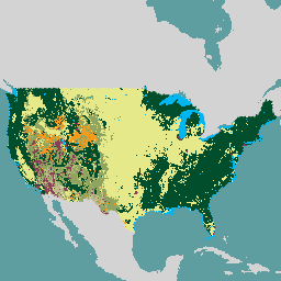
此产品是景观变化监测系统 (LCMS) 数据套件的一部分。该数据集显示了每年 LCMS 模式下的变化、土地覆盖和/或土地利用类别,涵盖美国本土 (CONUS) 以及 CONUS 以外的地区 (OCONUS),包括阿拉斯加 (AK)、波多黎各-美属维尔京群岛 (PRUSVI) 和夏威夷 (HAWAII)。
LCMS 是一种基于遥感技术的系统,用于绘制和监控美国各地的景观变化。其目标是开发一种一致的方法,利用最新的技术和变化检测方面的进展,制作出“最佳”地貌变化地图。
输出包括三种年度产品:变化、土地覆盖和土地利用。变化模型输出专门针对植被覆盖,包括缓慢损失、快速损失(也包括水文变化,例如淹没或干旱)和增加。这些值是针对 Landsat 时间序列的每一年预测的,是 LCMS 的基础产品。我们应用基于辅助数据集的规则集来创建最终的变化产品,该产品是对模型化变化进行细化/重新分类,将其分为 15 个类别,明确提供有关地貌变化原因的信息(例如,树木砍伐、野火、风灾)。土地覆被和土地利用地图描绘了每个年份的生命形式级土地覆被和广义级土地利用情况。
由于没有哪种算法在所有情况下都能表现出色,因此 LCMS 使用模型集成作为预测器,从而提高各种生态系统和变化过程中的地图准确性(Healey 等人,2018 年)。由此产生的一套 LCMS 变化、土地覆盖和土地利用地图可全面展示自 1985 年以来美国各地的地貌变化。
LCMS 模型的预测器层包括 LandTrendr 和 CCDC 变化检测算法的输出数据以及地形信息。而所有这些数据的获取与处理,均依托 Google Earth Engine 平台完成(Gorelick 等人,2017 年)。
为生成 LandTrendr 的年度合成影像,我们使用了 USGS Collection 2 Landsat Tier 1 和 Sentinel 2A、2B Level-1C 的大气层顶反射率数据。我们使用 cFmask 云遮罩算法(Foga 等人,2017 年)- Fmask 2.0(Zhu 和 Woodcock,2012 年)(仅限 Landsat)算法的一个实现、cloudScore(Chastain 等人,2019 年)(仅限 Landsat)、s2cloudless(Sentinel-Hub,2021 年)和 Cloud Score+(Pasquarella 等人,2023 年)(仅限 Sentinel 2)来遮盖云层;同时使用 TDOM(Chastain 等人,2019 年)来遮盖云影(Landsat 和 Sentinel 2)。对于 LandTrendr,我们会计算年度中心点 (annual medoid),将每年无云和无云影的像素值汇总成一幅单一的合成影像。对于 CCDC,我们使用了美国地质调查局 (USGS) Collection 2 Landsat Tier 1 地表反射率数据(针对美国本土),以及 Landsat Tier 1 大气层顶反射率数据(针对阿拉斯加、美属波多黎各和美属维尔京群岛以及夏威夷)。
我们使用 LandTrendr(Kennedy 等人,2010 年;Kennedy 等人,2018 年;Cohen 等人,2018 年)对合成时间序列进行时序分割。
所有无云和无云阴影的值也使用 CCDC 算法(Zhu 和 Woodcock,2014 年)进行时间分段。
预测变量数据包括原始合成值、LandTrendr 拟合值、成对差值、分段持续时间、变化幅度及斜率,以及 CCDC 正弦和余弦系数(前 3 个谐波)、拟合值和成对差值,连同源自 10 米 USGS 3D 高程计划 (3DEP) 数据(美国地质调查局,2019 年)的海拔、坡度、坡向正弦、坡向余弦和地形位置指数(Weiss,2001 年)。
参考数据是使用 TimeSync 收集的,这是一种基于 Web 的工具,可帮助分析师直观呈现和解读 1984 年至今的 Landsat 数据记录(Cohen 等人,2010 年)。
我们使用 TimeSync 中的参考数据以及 LandTrendr、CCDC 和地形指数中的预测器数据训练了随机森林模型 (Breiman, 2001),以预测年度变化、土地覆盖和土地利用类别。在建模之后,我们使用辅助数据集建立了一系列概率阈值和规则集,以改进定性地图输出并减少误报和漏报。如需了解详情,请参阅“说明”中包含的 LCMS 方法简介。
其他资源
LCMS Data Explorer 是一款基于 Web 的应用,可让用户查看、分析、总结和下载 LCMS 数据。
如需详细了解方法和精度评估结果,请参阅 LCMS 方法简介;如需下载数据、查看元数据和支持文档,请访问 LCMS 地理数据交换中心。
在即将发布的 v2025.11 数据版本中,字符串 HAWAII 将更新为 HI。
如有任何疑问或具体的数据请求,请发送邮件至 sm.fs.lcms@usda.gov。
频段
波段
像素大小:30 米(所有波段)
| 名称 | 像元大小 | 说明 | |||||||||||||||||||||||||||||||||||||||||||||||||||||||||||||||||||||||||||||||||||||||||||||||||
|---|---|---|---|---|---|---|---|---|---|---|---|---|---|---|---|---|---|---|---|---|---|---|---|---|---|---|---|---|---|---|---|---|---|---|---|---|---|---|---|---|---|---|---|---|---|---|---|---|---|---|---|---|---|---|---|---|---|---|---|---|---|---|---|---|---|---|---|---|---|---|---|---|---|---|---|---|---|---|---|---|---|---|---|---|---|---|---|---|---|---|---|---|---|---|---|---|---|---|---|
Change |
30 米 | 最终主题 LCMS 更改产品。每年总共映射了 15 个变化类别。从根本上讲,每个研究区域的变化都通过三个单独的二元随机森林模型进行建模:缓慢损失、快速损失和增加。每个像素都会分配给概率最高且高于指定阈值的模型变化类别。如果某个像素没有任何值高于相应类别的阈值,则会将其分配给“稳定”类别。根据使用模型化变化类别的规则集、辅助数据集(例如 TCC、MTBS 和 IDS)以及 LCMS 土地覆盖数据,将 15 个精细化变化原因类别之一分配给每个像素。如需详细了解规则集和所用的辅助数据集,请参阅“说明”中链接的 LCMS 方法简报。 |
|||||||||||||||||||||||||||||||||||||||||||||||||||||||||||||||||||||||||||||||||||||||||||||||||
Land_Cover |
30 米 | 最终的主题 LCMS 地表覆盖产品。我们每年都会使用 TimeSync 参考数据和从 Landsat 影像中提取的光谱信息,绘制总共 14 个土地覆盖类别的地图。地表覆盖是通过单个多类别随机森林模型预测的,该模型会输出一个数组,其中包含每个类别的概率(随机森林模型中“选择”每个类别的树的比例)。最终类别会分配给概率最高的土地用途。在分配概率最高的地表覆盖类别之前,根据研究区域,应用了一个或多个使用辅助数据集的概率阈值和规则集。如需详细了解概率阈值和规则集,请参阅说明中链接的 LCMS 方法简报。七个地表覆盖类别表示单一地表覆盖,其中地表覆盖类型覆盖了像素的大部分区域,而其他任何类别的覆盖面积均不超过像素的 10%。此外,还有 7 门混合课程。这些像素表示其他地表覆盖类别的覆盖率至少为 10% 的像素。 |
|||||||||||||||||||||||||||||||||||||||||||||||||||||||||||||||||||||||||||||||||||||||||||||||||
Land_Use |
30 米 | 最终专题 LCMS 土地利用产品。我们每年都会使用 TimeSync 参考数据和从 Landsat 影像中提取的光谱信息,绘制总共 5 个土地用途类别的地图。土地利用是使用单个多类别随机森林模型预测的,该模型会输出一个数组,其中包含每个类别的概率(随机森林模型中“选择”每个类别的树的比例)。最终类别会分配给概率最高的土地用途。在分配概率最高的地表覆盖类型之前,我们使用辅助数据集应用了一系列概率阈值和规则集。如需详细了解概率阈值和规则集,请参阅说明中链接的 LCMS 方法简报。 |
|||||||||||||||||||||||||||||||||||||||||||||||||||||||||||||||||||||||||||||||||||||||||||||||||
Change_Raw_Probability_Slow_Loss |
30 米 | 慢速损失的原始 LCMS 建模概率。“缓慢丢失”包括以下来自 TimeSync 更改流程解释的类别:
|
|||||||||||||||||||||||||||||||||||||||||||||||||||||||||||||||||||||||||||||||||||||||||||||||||
Change_Raw_Probability_Fast_Loss |
30 米 | 快速损失的原始 LCMS 建模概率。快速丢失包括以下来自 TimeSync 更改流程解释的类:
|
|||||||||||||||||||||||||||||||||||||||||||||||||||||||||||||||||||||||||||||||||||||||||||||||||
Change_Raw_Probability_Gain |
30 米 | 增益的原始 LCMS 建模概率。定义为:由于生长和演替,植被覆盖率在一年或多年内增加的土地。适用于可能表现出与植被再生相关的光谱变化的任何区域。在发达地区,增长可能源于成熟的植被和/或新安装的草坪和景观。在森林中,生长包括从裸露地面开始的植被生长,以及中等高度和共同优势树木和/或低矮的草和灌木的生长。在森林采伐后记录的增长/恢复区段可能会随着森林的再生而经历不同的土地覆盖类别。只有当光谱值与持续数年的上升趋势线(例如,如果延伸到约 20 年,斜率为正且 NDVI 值约为 0.10 单位)密切相关时,这些变化才会被视为增长/恢复。 |
|||||||||||||||||||||||||||||||||||||||||||||||||||||||||||||||||||||||||||||||||||||||||||||||||
Land_Cover_Raw_Probability_Trees |
30 米 | 树木的原始 LCMS 建模概率。定义为:像素的大部分由活树或枯立木组成。 |
|||||||||||||||||||||||||||||||||||||||||||||||||||||||||||||||||||||||||||||||||||||||||||||||||
Land_Cover_Raw_Probability_Tall-Shrubs-and-Trees-Mix |
30 米 | 高灌木和树木混合(仅限阿拉斯加)的原始 LCMS 建模概率。定义为:像素的大部分由高度超过 1 米的灌木组成,并且至少包含 10% 的活树或枯立木。 |
|||||||||||||||||||||||||||||||||||||||||||||||||||||||||||||||||||||||||||||||||||||||||||||||||
Land_Cover_Raw_Probability_Shrubs-and-Trees-Mix |
30 米 | 灌木和树木混合的原始 LCMS 建模概率。定义为:像素的大部分由灌木组成,并且至少有 10% 由活树或枯立木组成。 |
|||||||||||||||||||||||||||||||||||||||||||||||||||||||||||||||||||||||||||||||||||||||||||||||||
Land_Cover_Raw_Probability_Grass-Forb-Herb-and-Trees-Mix |
30 米 | 草类/草本植物和树木混合的原始 LCMS 建模概率。定义为:像素的大部分由多年生草、草本植物或其他草本植被组成,并且至少有 10% 的活树或枯立木。 |
|||||||||||||||||||||||||||||||||||||||||||||||||||||||||||||||||||||||||||||||||||||||||||||||||
Land_Cover_Raw_Probability_Barren-and-Trees-Mix |
30 米 | 贫瘠土地和树木混合的原始 LCMS 建模概率。定义为:像素的大部分由扰动暴露的裸土(例如,机械清理或森林采伐暴露的土壤)以及常年贫瘠的区域(例如沙漠、干盐湖、露岩地(包括因地表采矿活动而暴露的矿物和其他地质材料)、沙丘、盐碱滩和海滩)组成。由泥土和碎石铺成的道路也被视为贫瘠土地,并且至少包含 10% 的活树或枯立木。 |
|||||||||||||||||||||||||||||||||||||||||||||||||||||||||||||||||||||||||||||||||||||||||||||||||
Land_Cover_Raw_Probability_Tall-Shrubs |
30 米 | 高灌木(仅限阿拉斯加)的原始 LCMS 建模概率。定义为:像素的大部分由高度超过 1 米的灌木组成。 |
|||||||||||||||||||||||||||||||||||||||||||||||||||||||||||||||||||||||||||||||||||||||||||||||||
Land_Cover_Raw_Probability_Shrubs |
30 米 | 灌木的原始 LCMS 建模概率。定义为:像素的大部分由灌木组成。 |
|||||||||||||||||||||||||||||||||||||||||||||||||||||||||||||||||||||||||||||||||||||||||||||||||
Land_Cover_Raw_Probability_Grass-Forb-Herb-and-Shrubs-Mix |
30 米 | 草类/禾草类/草本植物和灌木混合物的原始 LCMS 建模概率。定义为:像素的大部分由多年生草、草本植物或其他草本植被组成,并且至少有 10% 由灌木组成。 |
|||||||||||||||||||||||||||||||||||||||||||||||||||||||||||||||||||||||||||||||||||||||||||||||||
Land_Cover_Raw_Probability_Barren-and-Shrubs-Mix |
30 米 | 贫瘠和灌木混合的原始 LCMS 建模概率。定义为:像素的大部分由扰动暴露的裸土(例如,机械清理或森林采伐暴露的土壤)以及常年贫瘠的区域(例如沙漠、干盐湖、露岩地(包括因地表采矿活动而暴露的矿物和其他地质材料)、沙丘、盐碱滩和海滩)组成。由泥土和碎石铺成的道路也被视为贫瘠土地,并且至少包含 10% 的灌木。 |
|||||||||||||||||||||||||||||||||||||||||||||||||||||||||||||||||||||||||||||||||||||||||||||||||
Land_Cover_Raw_Probability_Grass-Forb-Herb |
30 米 | 草/禾草/草本植物的原始 LCMS 建模概率。定义为:像素的大部分由多年生草、草本植物或其他形式的草本植被组成。 |
|||||||||||||||||||||||||||||||||||||||||||||||||||||||||||||||||||||||||||||||||||||||||||||||||
Land_Cover_Raw_Probability_Barren-and-Grass-Forb-Herb-Mix |
30 米 | 贫瘠土地和草/禾草/草本植物混合物的原始 LCMS 建模概率。定义为:像素的大部分由扰动暴露的裸露土壤(例如,机械清理或森林采伐后暴露的土壤)以及常年贫瘠的区域(例如沙漠、干盐湖、岩石露头 [包括地表采矿活动暴露的矿物和其他地质材料]、沙丘、盐碱滩和海滩)组成。由泥土和碎石铺成的道路也被视为贫瘠土地,并且至少包含 10% 的多年生草、草本植物或其他草本植被。 |
|||||||||||||||||||||||||||||||||||||||||||||||||||||||||||||||||||||||||||||||||||||||||||||||||
Land_Cover_Raw_Probability_Barren-or-Impervious |
30 米 | 贫瘠或不透水地表的原始 LCMS 建模概率。定义为:像素的大部分由以下部分组成:1.) 因扰动而暴露的裸土(例如因机械清理或森林采伐而暴露的土壤),以及常年贫瘠的区域,例如沙漠、干盐湖、露岩(包括因地表采矿活动而暴露的矿物和其他地质材料)、沙丘、盐碱滩和海滩。由泥土和碎石铺成的道路也被视为贫瘠的土地;2.) 水无法渗透的人造材料,例如铺砌的道路、屋顶和停车场。 |
|||||||||||||||||||||||||||||||||||||||||||||||||||||||||||||||||||||||||||||||||||||||||||||||||
Land_Cover_Raw_Probability_Snow-or-Ice |
30 米 | 雪或冰的原始 LCMS 建模概率。定义为:大部分像素由雪或冰组成。 |
|||||||||||||||||||||||||||||||||||||||||||||||||||||||||||||||||||||||||||||||||||||||||||||||||
Land_Cover_Raw_Probability_Water |
30 米 | 水的原始 LCMS 建模概率。定义为:像素的大部分由水组成。 |
|||||||||||||||||||||||||||||||||||||||||||||||||||||||||||||||||||||||||||||||||||||||||||||||||
Land_Use_Raw_Probability_Agriculture |
30 米 | 农业的原始 LCMS 建模概率。定义为:用于生产食物、纤维和燃料的土地,处于植被覆盖状态或无植被状态。这包括但不限于耕种和未耕种的农田、草地、果园、葡萄园、圈养牲畜作业区,以及种植水果、坚果或浆果的生产区。 主要用于农业用途(即不用于城镇间的公共交通)的道路被视为农业用地。 |
|||||||||||||||||||||||||||||||||||||||||||||||||||||||||||||||||||||||||||||||||||||||||||||||||
Land_Use_Raw_Probability_Developed |
30 米 | “发达”的原始 LCMS 建模概率。定义为:被人造结构(例如高密度住宅、商业、工业、采矿或交通)覆盖的土地,或植被(包括树木)和结构(例如低密度住宅、草坪、休闲设施、墓地、交通和公用事业走廊等)的混合体,包括因人类活动而发生功能性改变的任何土地。 |
|||||||||||||||||||||||||||||||||||||||||||||||||||||||||||||||||||||||||||||||||||||||||||||||||
Land_Use_Raw_Probability_Forest |
30 米 | 森林的原始 LCMS 建模概率。定义为:已种植或自然植被覆盖的土地,在近期演替序列中的某个时间点,其树木覆盖率达到(或可能达到)10% 或更高。这可能包括天然森林、人工林和木本湿地的落叶、常绿和/或混合类别。 |
|||||||||||||||||||||||||||||||||||||||||||||||||||||||||||||||||||||||||||||||||||||||||||||||||
Land_Use_Raw_Probability_Other |
30 米 | 其他类别的原始 LCMS 建模概率。定义为:根据光谱趋势或其他支持性证据,土地(无论用途如何)上发生了扰动或变化事件,但无法确定确切原因,或者变化类型不符合上述任何变化过程类别。 |
|||||||||||||||||||||||||||||||||||||||||||||||||||||||||||||||||||||||||||||||||||||||||||||||||
Land_Use_Raw_Probability_Rangeland-or-Pasture |
30 米 | 草原或牧场的原始 LCMS 建模概率。定义为:此类包含以下任何区域:a.) 牧草地,其中植被是本地草类、灌木、草本植物和类草植物的混合体,主要由降雨、温度、海拔和火灾等自然因素和过程产生,尽管有限的管理可能包括规定燃烧以及家养和野生草食动物的放牧;或 b.) 牧场,植被可能包括混合的、主要为天然的草类、草本植物和药草,也可能包括经过管理、以播种和管理来维持近乎单一栽培的草类为主的植被。 |
|||||||||||||||||||||||||||||||||||||||||||||||||||||||||||||||||||||||||||||||||||||||||||||||||
QA_Bits |
30 米 | 有关年度 LCMS 产品输出值来源的辅助信息。 |
|||||||||||||||||||||||||||||||||||||||||||||||||||||||||||||||||||||||||||||||||||||||||||||||||
更改类别表
| 值 | 颜色 | 说明 |
|---|---|---|
| 1 | #ff09f3 | Wind |
| 2 | #541aff | 飓风 |
| 3 | #e4f5fd | 雪或冰转场效果 |
| 4 | #cc982e | 干燥 |
| 5 | #0adaff | 洪灾 |
| 6 | #a10018 | 计划烧除 |
| 7 | #d54309 | Wildfire |
| 8 | #fafa4b | 机械土地改造 |
| 9 | #afde1c | 移除树木 |
| 10 | #ffc80d | 落叶 |
| 11 | #a64c28 | 南方松树皮甲 |
| 12 | #f39268 | 虫害、病害或干旱胁迫 |
| 13 | #c291d5 | 其他损失 |
| 14 | #00a398 | 植被演替生长 |
| 15 | #3d4551 | 稳定 |
| 16 | #1b1716 | 非处理区域遮罩 |
Land_Cover 类表
| 值 | 颜色 | 说明 |
|---|---|---|
| 1 | #004e2b | 树 |
| 2 | #009344 | 高灌木和树木混合 (仅限 AK) |
| 3 | #61bb46 | 灌木和树木混合 |
| 4 | #acbb67 | 草/草本植物/香草和树木混合 |
| 5 | #8b8560 | 荒地与树木混搭 |
| 6 | #cafd4b | 高灌木(仅限 AK) |
| 7 | #f89a1c | 灌木 |
| 8 | #8fa55f | 草类/草本植物/灌木混合 |
| 9 | #bebb8e | 贫瘠土地和灌木丛合辑 |
| 10 | #e5e98a | 草类/草本植物/香草 |
| 11 | #ddb925 | 贫瘠土地和草/多年生草本植物/草本植物混合 |
| 12 | #893f54 | 贫瘠或不透水 |
| 13 | #e4f5fd | 下雪或结冰 |
| 14 | #00b6f0 | 水 |
| 15 | #1b1716 | 非处理区域遮罩 |
Land_Use 类别表
| 值 | 颜色 | 说明 |
|---|---|---|
| 1 | #fbff97 | 农业 |
| 2 | #e6558b | 开发 |
| 3 | #004e2b | 森林 |
| 4 | #9dbac5 | 其他 |
| 5 | #a6976a | 草地或牧场 |
| 6 | #1b1716 | 非处理区域遮罩 |
图片属性
图像属性
| 名称 | 类型 | 说明 |
|---|---|---|
| study_area | STRING | 此 LCMS 版本涵盖美国本土、阿拉斯加、波多黎各-美属维尔京群岛和夏威夷。 可能的值:'CONUS, AK, PRUSVI, HAWAII' |
| 版本 | STRING | 产品版本 |
| startYear | INT | 产品的起始年份 |
| endYear | INT | 产品的结束年份 |
| 年 | INT | 产品年份 |
使用条款
使用条款
美国农业部林务局不作任何明示或暗示的保证,包括对适销性和特定用途适用性的保证,也不对这些地理空间数据的准确性、可靠性、完整性或效用承担任何法律责任或义务,或因不当或不正确使用这些地理空间数据而产生的后果承担任何法律责任或义务。这些地理空间数据及相关地图或图形并非法律文件,也不得用作法律文件。不得使用这些数据和地图来确定产权、所有权、法律说明或边界、法律管辖权,或可能对公共土地或私人土地施加的限制。 数据和地图可能未标示自然灾害,土地使用者应谨慎行事。数据是动态的,可能随时间变化。用户有责任核实地理空间数据的局限性,并据此使用数据。
这些数据由美国政府资助收集,无需额外许可或费用即可使用。如果您在出版物、演示文稿或其他研究产品中使用这些数据,请按如下格式引用:
美国农业部林务局。2025 年。美国林务局景观变化监测系统 v2024.10(美国本土和美国本土以外的美国本土)。犹他州盐湖城。
引用
美国农业部林务局。2025 年。美国林务局景观变化监测系统 v2024.10(美国本土和美国本土外)。犹他州盐湖城。
Breiman, L.,2001 年。随机森林。刊载于《机器学习》栏目。Springer,45:5-32。 doi:10.1023/A:1010933404324
Chastain, R.、Housman, I.、Goldstein, J.、Finco, M. 和 Tenneson, K.,2019 年。 针对美国本土上空的 Sentinel-2A 和 2B MSI、Landsat-8 OLI 及 Landsat-7 ETM 传感器的跨传感器大气层顶光谱特性实证比较。刊载于《环境遥感》期刊。Science Direct,221:274-285。doi:10.1016/j.rse.2018.11.012
Cohen, W. B., Yang, Z. 和 Kennedy, R.,2010 年。使用年度 Landsat 时序数据检测森林扰动和恢复趋势:2. TimeSync - 用于校准和验证的工具。刊载于《环境遥感》期刊。Science Direct,114(12):2911-2924。doi:10.1016/j.rse.2010.07.010
Cohen, W. B.、Yang, Z.、Healey, S. P.、Kennedy, R. E. 和 Gorelick, N., 2018 年。一种用于森林扰动检测的 LandTrendr 多光谱集成方法。刊载于《环境遥感》期刊。Science Direct,205:131-140。 doi:10.1016/j.rse.2017.11.015
Foga, S.、Scaramuzza, P.L.、Guo, S.、Zhu, Z.、Dilley, R.D.、Beckmann, T.、Schmidt, G.L.、Dwyer, J.L.、Hughes, M.J.、Laue, B.,2017 年。面向业务化 Landsat 数据产品的云检测算法比较与验证。刊载于《环境遥感》期刊。Science Direct,194:379-390。 doi:10.1016/j.rse.2017.03.026
美国地质调查局,2019 年。USGS 3D 高程计划数字高程模型,于 2022 年 8 月访问,网址为 https://developers.google.com/earth-engine/datasets/catalog/USGS_3DEP_10m
Healey, S. P. Cohen, W. B.、Yang, Z.、Kenneth Brewer, C.、Brooks, E. B., Gorelick, N.、Hernandez, A. J. Huang, C.、Joseph Hughes, M.、Kennedy, R. E., Loveland, T. R., Moisen, G. G. Schroeder, T. A., Stehman, S. V., Vogelmann, J. E., Woodcock, C. E., Yang, L. 和 Zhu, Z.,2018 年。使用堆叠泛化方法绘制森林变化图:一种集成方法。刊载于《环境遥感》期刊。Science Direct,204:717-728。 doi:10.1016/j.rse.2017.09.029
Kennedy, R. E.、Yang, Z. 和 Cohen, W. B., 2010 年。使用年度 Landsat 时序数据检测森林扰动和恢复趋势:1.LandTrendr - 时间分割算法。刊载于《环境遥感》期刊。Science Direct,114(12):2897-2910。doi:10.1016/j.rse.2010.07.008
Kennedy, R.、Yang, Z.、Gorelick, N.、Braaten, J.、Cavalcante, L.、 Cohen, W. 和 Healey, S. 2018 年。在 Google Earth Engine 上实现 LandTrendr 算法。刊载于《遥感》期刊。MDPI,10(5):691。doi:10.3390/rs10050691
Pasquarella, V. J., Brown, C. F.、Czerwinski, W. 和 Rucklidge, W. J. 2023 年。 使用弱监督视频学习对光学卫星图像进行全面质量评估。收录于《IEEE/CVF 计算机视觉与模式识别会议论文集》。2124-2134。
Sentinel-Hub,2021 年。Sentinel 2 Cloud Detector。[在线]。可在以下网址获取: https://github.com/sentinel-hub/sentinel2-cloud-detector
Weiss, A.D.、2001 年。地形位置和地貌分析,海报展示,ESRI 用户大会,加利福尼亚州圣地亚哥,Zhu, Z., 和 Woodcock, C. E. 2012。Landsat 影像中基于对象的云与云影检测。118:83-94。
Zhu, Z. 和 Woodcock, C. E., 2012。Landsat 影像中基于对象的云与云影检测。刊载于《环境遥感》期刊。Science Direct,118:83-94。doi:10.1016/j.rse.2011.10.028
Zhu, Z. 和 Woodcock, C. E., 2014 年。使用所有可用的 Landsat 数据持续检测和分类土地覆盖。 刊载于《环境遥感》期刊。Science Direct,144:152-171。 doi:10.1016/j.rse.2014.01.011
DOI
- https://doi.org/10.1016/j.rse.2010.07.008
- https://doi.org/10.1016/j.rse.2010.07.010
- https://doi.org/10.1016/j.rse.2011.10.028
- https://doi.org/10.1016/j.rse.2014.01.011
- https://doi.org/10.1016/j.rse.2017.03.026
- https://doi.org/10.1016/j.rse.2017.09.029
- https://doi.org/10.1016/j.rse.2017.11.015
- https://doi.org/10.1016/j.rse.2018.11.012
- https://doi.org/10.1023/A:1010933404324
- https://doi.org/10.3390/rs10050691
通过 Earth Engine 探索
代码编辑器 (JavaScript)
var dataset = ee.ImageCollection('USFS/GTAC/LCMS/v2024-10');

var lcms = dataset.filterDate('2022', '2023')  // range: [1985, 2024]
               .filter('study_area == "CONUS"')  // "AK", "HAWAII", "PRUSVI"
               .first();

Map.addLayer(lcms.select('Land_Cover'), {}, 'Land Cover');
Map.addLayer(lcms.select('Land_Use'), {}, 'Land Use');
Map.addLayer(lcms.select('Change'), {}, 'Vegetation Change', false);

Map.setCenter(-98.58, 38.14, 4);