수동으로 결합된 지형지물 데이터를 비교하는 대신 지형지물 데이터를 임베딩이라는 표현으로 축소한 다음 임베딩을 비교할 수 있습니다. 임베딩은 특성 데이터 자체에 대해 감독 심층신경망 (DNN)을 학습시켜 생성됩니다. 임베딩은 일반적으로 특징 데이터보다 크기가 작은 임베딩 공간의 벡터에 특징 데이터를 매핑합니다. 임베딩은 머신러닝 단기집중과정 임베딩 모듈에서 다루고 신경망은 신경망 모듈에서 다룹니다. 유사한 예시의 임베딩 벡터(예: 동일한 사용자가 시청한 유사한 주제의 YouTube 동영상)는 임베딩 공간에서 서로 가까워집니다. 감독 유사성 측정값은 이 '근접성'을 사용하여 예시 쌍의 유사성을 수치화합니다.
유사성 측정을 만들기 위해 감독 학습에 관해만 논의하고 있습니다. 수동이든 감독이든 유사성 측정값은 알고리즘에서 비지도 클러스터링을 실행하는 데 사용됩니다.
수동 측정과 감독 측정 비교
이 표에서는 요구사항에 따라 수동 또는 감독 유사성 측정항목을 사용해야 하는 경우를 설명합니다.
요구사항
수동
감독 대상
상관된 지형지물에서 중복 정보를 제거합니다.
아니요. 특성 간의 상관관계를 조사해야 합니다.
예, DNN은 중복 정보를 제거합니다.
계산된 유사성에 대한 통계를 제공합니다.
예
아니요. 임베딩은 복호화할 수 없습니다.
기능이 적은 소규모 데이터 세트에 적합한가요?
예.
아니요. 소규모 데이터 세트는 DNN에 충분한 학습 데이터를 제공하지 않습니다.
기능이 많은 대규모 데이터 세트에 적합한가요?
아니요. 여러 지형지물에서 중복 정보를 수동으로 삭제한 다음 결합하는 것은 매우 어렵습니다.
예. DNN은 중복 정보를 자동으로 제거하고 기능을 결합합니다.
감독 유사성 측정 생성
다음은 감독된 유사성 측정값을 만드는 절차에 대한 개요입니다.
그림 1: 감독 유사성 측정항목을 만드는 단계
이 페이지에서는 DNN에 대해 설명하고 다음 페이지에서는 나머지 단계를 설명합니다.
학습 라벨을 기반으로 DNN 선택
동일한 특성 데이터를 입력과 라벨로 모두 사용하는 DNN을 학습하여 특성 데이터를 더 낮은 차원의 임베딩으로 줄입니다. 예를 들어 주택 데이터의 경우 DNN은 가격, 크기, 우편번호와 같은 특성을 사용하여 이러한 특성 자체를 예측합니다.
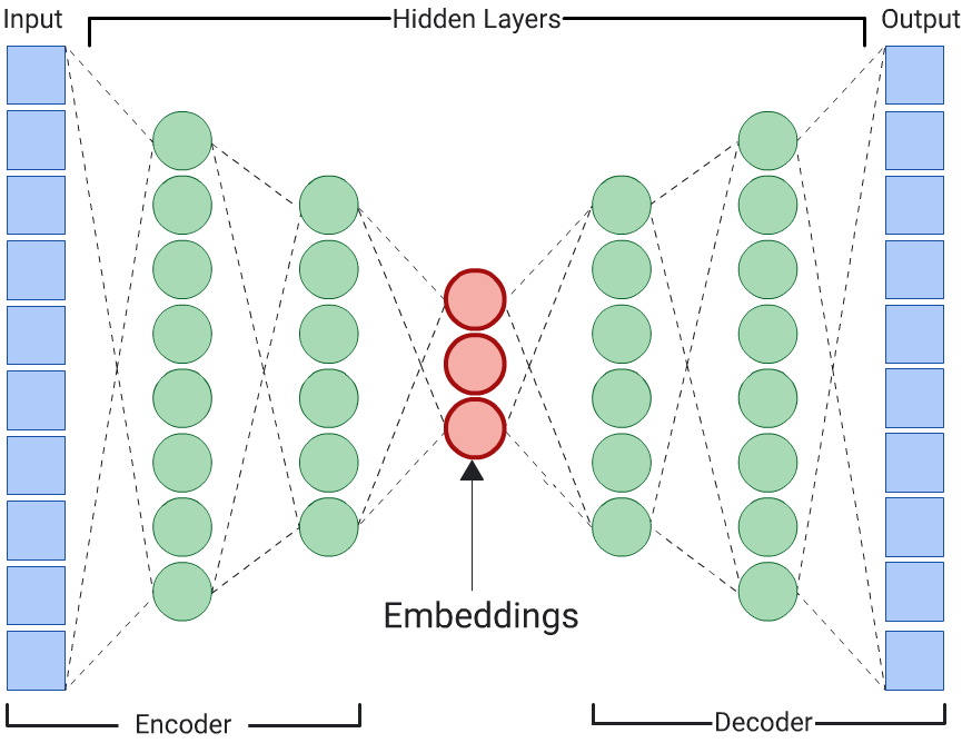
Autoencoder
입력 데이터 자체를 예측하여 입력 데이터의 임베딩을 학습하는 DNN을 오토인코더라고 합니다.
자동 인코더의 숨겨진 레이어는 입력 및 출력 레이어보다 작으므로 자동 인코더는 입력 특성 데이터의 압축된 표현을 학습해야 합니다. DNN이 학습되면 가장 작은 숨겨진 레이어에서 임베딩을 추출하여 유사성을 계산합니다.
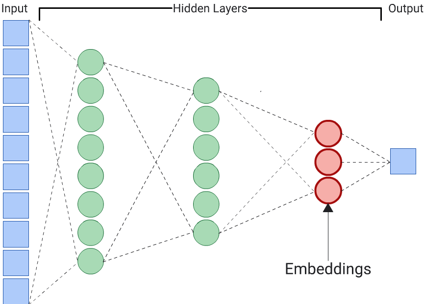
그림 2: 자동 인코더 아키텍처
예측자
자동 인코더는 임베딩을 생성하는 가장 간단한 방법입니다. 그러나 유사성을 판단할 때 특정 기능이 다른 기능보다 더 중요할 수 있는 경우에는 자동 인코더가 최적의 선택이 아닙니다. 예를 들어 주택 데이터에서 가격이 우편번호보다 중요하다고 가정합니다. 이 경우 중요한 특성만 DNN의 학습 라벨로 사용합니다. 이 DNN은 모든 입력 특성을 예측하는 대신 특정 입력 특성을 예측하므로 예측자 DNN이라고 합니다. 임베딩은 일반적으로 마지막 임베딩 레이어에서 추출해야 합니다.
그림 3: 예측자 아키텍처
라벨로 사용할 지형지물을 선택할 때는 다음 사항을 고려하세요.
숫자 특성의 경우 손실을 더 쉽게 계산하고 해석할 수 있으므로 범주형 특성보다 숫자 특성을 사용하는 것이 좋습니다.
DNN의 입력에서 라벨로 사용하는 특성을 삭제합니다. 그러지 않으면 DNN이 해당 특성을 사용하여 출력을 완벽하게 예측합니다. 이는 라벨 유출의 극단적인 예입니다.
[null,null,["최종 업데이트: 2025-02-25(UTC)"],[[["\u003cp\u003eSupervised similarity measures leverage deep neural networks (DNNs) to learn embeddings, which are lower-dimensional representations of feature data, for comparing items like YouTube videos.\u003c/p\u003e\n"],["\u003cp\u003eUnlike manual similarity measures, supervised measures excel with large datasets and automatically handle redundant information, but they lack the interpretability of manual methods.\u003c/p\u003e\n"],["\u003cp\u003eTo create a supervised similarity measure, you train a DNN (either an autoencoder predicting its own input or a predictor focusing on key features) to generate embeddings that capture item similarity.\u003c/p\u003e\n"],["\u003cp\u003eWhen designing the DNN, prioritize numerical features as labels and avoid label leakage by removing the label feature from the input data.\u003c/p\u003e\n"],["\u003cp\u003eEmbeddings from similar items will be clustered closer together in the embedding space, allowing for similarity comparisons using distance-based metrics.\u003c/p\u003e\n"]]],[],null,["Instead of comparing manually-combined feature data, you can reduce the feature\ndata to representations called\n[**embeddings**](/machine-learning/glossary#embeddings), then compare the\nembeddings. Embeddings are generated by training a supervised [**deep neural\nnetwork**](/machine-learning/glossary#neural_network) (**DNN** ) on the feature\ndata itself. The embeddings map the feature data to a vector in an embedding\nspace with typically fewer dimensions than the feature data. Embeddings are\ndiscussed in the [Embeddings](/machine-learning/crash-course/embeddings)\nmodule of Machine Learning Crash Course, while neural nets are discussed in the\n[Neural nets](/machine-learning/crash-course/neural-networks)\nmodule. Embedding vectors for similar examples, such as YouTube videos on\nsimilar topics watched by the same users, end up close together in the embedding\nspace. A **supervised similarity measure**\nuses this \"closeness\" to quantify the similarity for pairs of\nexamples.\n\nRemember, we're discussing supervised learning only to create our similarity\nmeasure. The similarity measure, whether manual or supervised, is then used by\nan algorithm to perform unsupervised clustering.\n\nComparison of Manual and Supervised Measures\n\nThis table describes when to use a manual or supervised similarity\nmeasure depending on your requirements.\n\n| Requirement | Manual | Supervised |\n|----------------------------------------------------------|------------------------------------------------------------------------------------------------------------------|------------------------------------------------------------------------------------|\n| Eliminates redundant information in correlated features? | No, you need to investigate any correlations between features. | Yes, DNN eliminates redundant information. |\n| Gives insight into calculated similarities? | Yes | No, embeddings cannot be deciphered. |\n| Suitable for small datasets with few features? | Yes. | No, small datasets don't provide enough training data for a DNN. |\n| Suitable for large datasets with many features? | No, manually eliminating redundant information from multiple features and then combining them is very difficult. | Yes, the DNN automatically eliminates redundant information and combines features. |\n\nCreating a supervised similarity measure\n\nHere's an overview of the process to create a supervised similarity measure:\n**Figure 1: Steps to create a supervised similarity\nmeasure.**\n\nThis page discusses DNNs, while\nthe following pages cover the remaining steps.\n\nChoose DNN based on training labels\n\nReduce your feature data to lower-dimensional embeddings by training a DNN that\nuses the same feature data both as input and as the labels. For example, in\nthe case of house data, the DNN would use the features---such as price, size, and\npostal code---to predict those features themselves.\n\nAutoencoder\n\nA DNN that learns embeddings of input data by predicting the input data itself\nis called an [autoencoder](/machine-learning/glossary#autoencoder).\nBecause an autoencoder's hidden layers are smaller\nthan the input and output layers, the autoencoder is forced to learn a\ncompressed representation of the input feature data. Once the DNN is trained,\nextract the embeddings from the smallest hidden layer to calculate similarity.\n**Figure 2: Autoencoder architecture.**\n\nPredictor\n\nAn autoencoder is the simplest choice to generate embeddings. However, an\nautoencoder isn't the optimal choice when certain features could be more\nimportant than others in determining similarity. For example, in house data,\nassume price is more important than postal code. In such cases, use\nonly the important feature as the training label for the DNN. Since this DNN\npredicts a specific input feature instead of predicting all input features, it\nis called a **predictor** DNN. Embeddings should usually be extracted from the\nlast embedding layer.\n**Figure 3: Predictor architecture.**\n\nWhen choosing a feature to be the label:\n\n- Prefer numerical to categorical features because loss\n is easier to calculate and interpret for numeric features.\n\n- Remove the feature that you use as the label from the input to the DNN, or\n else the DNN will use that feature to perfectly predict the output. (This is\n an extreme example of [label leakage](/machine-learning/glossary#label-leakage).)\n\nDepending on your choice of labels, the resulting DNN is either an\nautoencoder or a predictor.\n| **Key terms:**\n|\n| - [embeddings](/machine-learning/glossary#embeddings)\n| - [Deep Neural Network (DNN)](/machine-learning/glossary#neural_network)"]]