本部分将回顾机器学习速成课程的处理数值数据模块中与聚类最相关的数据准备步骤。
在聚类中,您可以通过将两个示例的所有特征数据组合成一个数值来计算两个示例之间的相似性。这要求特征具有相同的尺度,这可以通过标准化、转换或创建百分位数来实现。如果您想转换数据,但不检查其分布情况,可以默认使用百分位数。
对数据进行归一化
您可以通过对数据进行标准化,将多个特征的数据转换为相同的尺度。
Z 分
每当您看到数据集大致呈现正态分布的形状时,都应为数据计算z 分数。Z 得分是指某个值与平均值之间的标准差数量。如果数据集不够大,无法使用百分位数,您也可以使用 z 分数。
如需查看相关步骤,请参阅Z 分标准化。
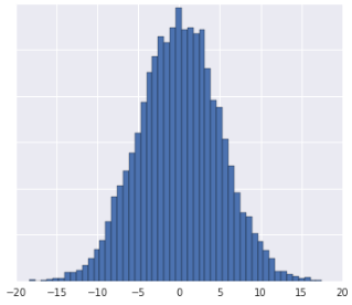
下面的可视化图展示了数据集的两个特征在进行 Z 得分标准化之前和之后的变化情况:

在左侧未归一化的数据集中,特征 1 和特征 2 分别在 x 轴和 y 轴上绘制,但它们的刻度不同。在左侧,红色示例与蓝色更接近或更相似,而与黄色更不接近或不相似。在右侧,经过 Z 分标准化后,特征 1 和特征 2 具有相同的尺度,并且红色示例看起来更接近黄色示例。标准化数据集可更准确地衡量点之间的相似性。
日志转换
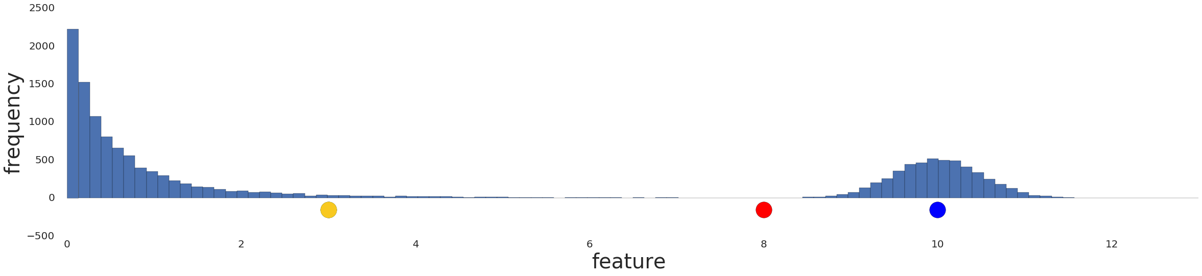
如果数据集完全符合幂律分布(即数据在最低值处严重重合),请使用对数转换。如需查看相关步骤,请参阅日志扩缩。
下面是对对数转换前后幂律数据集的可视化结果:

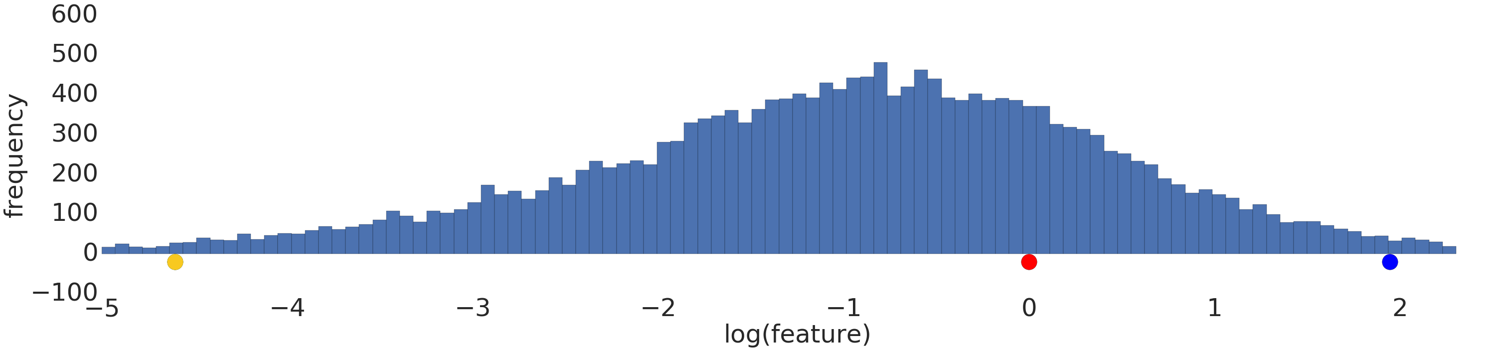
在日志缩放之前(图 2),红色示例看起来更像黄色。对日志进行缩放后(图 3),红色看起来更接近蓝色。
分位数
当数据集不符合已知分布时,将数据分箱为百分位数效果很好。例如,以下数据集:
直观地讲,如果两个示例之间只有少数示例(无论其值如何),则这两个示例更相似;如果两个示例之间有许多示例,则这两个示例更不相似。通过上方的可视化结果,很难看出介于红色和黄色之间或介于红色和蓝色之间的示例总数。
我们可以通过将数据集划分为四分位数(即每个包含相同数量示例的区间),并为每个示例分配四分位数索引,来获得对相似性的这种理解。如需查看相关步骤,请参阅百分位分桶。
下面是将上一个分布划分为四分位数的分布图,显示红色与黄色相差一个四分位数,与蓝色相差三个四分位数:
![一张图表,显示转换为百分位数后的数据。线条表示 20 个间隔。]](https://developers.google.cn/static/machine-learning/clustering/images/Quantize.png?authuser=5&hl=ca)
您可以选择任意数量的百分位数。 \(n\) 不过,为了让百分位数能够有意义地代表基础数据,您的数据集应至少包含\(10n\) 个示例。如果您没有足够的数据,请改为进行标准化。
检查您的理解情况
对于以下问题,假设您有足够的数据来创建百分位数。
问题 1

- 数据分布为高斯分布。
- 您对数据在真实世界中的含义有了一些了解,这表明数据不应进行非线性转换。
问题二
缺少数据
如果您的数据集中存在缺少某个特征值的示例,但这些示例很少出现,您可以移除这些示例。如果这些示例经常出现,您可以完全移除该特征,也可以使用机器学习模型根据其他示例预测缺失的值。例如,您可以使用基于现有特征数据训练的回归模型对缺失的数值数据进行插值。