本頁面由 Cloud Translation API 翻譯而成。

Dynamic World V1

資料集可用性: 2015-06-27T00:00:00Z–2025-03-09T03:20:17Z
資料集供應器: World Resources Institute Google
Earth Engine 程式碼片段: ee.ImageCollection("GOOGLE/DYNAMICWORLD/V1")

標記: global google landcover landuse nrt sentinel2-derived

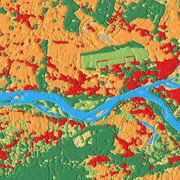
Dynamic World 是 10 公尺近乎即時 (NRT) 的土地使用/土地覆蓋 (LULC) 資料集，包含九個類別的類別機率和標籤資訊。

動態世界預測功能適用於 2015 年 6 月 27 日至目前的 Sentinel-2 L1C 集合。Sentinel-2 的回訪頻率介於 2 到 5 天，具體取決於緯度。系統會針對 CLOUDY_PIXEL_PERCENTAGE <= 35% 的 Sentinel-2 L1C 圖像產生動態世界預測資料。系統會使用 S2 雲端機率、雲端位移指數和方向距離轉換的組合，遮蓋預測結果，以移除雲端和雲端陰影。

Dynamic World 集合中的圖片名稱，會與擷取圖片的 Sentinel-2 L1C 素材資源名稱相符，例如：

ee.Image('COPERNICUS/S2/20160711T084022_20160711T084751_T35PKT')

有相符的動態世界圖片，名稱為： ee.Image('GOOGLE/DYNAMICWORLD/V1/20160711T084022_20160711T084751_T35PKT')。

除了「標籤」頻帶以外，所有機率頻帶加總起來的值為 1。

如要進一步瞭解 Dynamic World 資料集，並查看產生組合、計算區域統計資料和使用時間序列的範例，請參閱「Dynamic World 簡介」教學課程系列。

由於 Dynamic World 類別估計值是根據單張圖片，使用小型移動視窗的空間背景而得出，因此如果預測的土地覆蓋率部分由時間上的覆蓋率所定義 (例如農作物)，在沒有明顯區別特徵的情況下，前 1 個「機率」可能會相對較低。在乾燥氣候中，沙子、陽光反射等高反光表面也可能會出現這種現象。

如要只選取確實屬於動態世界類別的像素，建議您設定閾值，以便根據前 1 項預測的預估「機率」遮罩動態世界輸出結果。

像素大小
10 公尺

錶帶

名稱	最大值	說明
`water`	1	預估完全浸水的機率
`trees`	1	樹木完全遮蔽的預估機率
`grass`	1	草地完全覆蓋的預估機率
`flooded_vegetation`	1	淹水植物完全覆蓋的預估機率
`crops`	1	預估裁剪區域完全涵蓋的機率
`shrub_and_scrub`	1	灌木和灌叢完全覆蓋的預估機率
`built`	1	預估建構完成的涵蓋率
`bare`	1	預估使用 bare 達到完整涵蓋率的機率
`snow_and_ice`	1	預估雪和冰覆蓋率
`label`	8	估計機率最高的頻帶索引

標籤類別表格

值	顏色	說明
0	#419bdf	水
1	#397d49	樹木
2	#88b053	青草
3	#7a87c6	flooded_vegetation
4	#e49635	作物
5	#dfc35a	shrub_and_scrub
6	#c4281b	已建構
7	#a59b8f	裸露
8	#b39fe1	snow_and_ice

圖片屬性

名稱	類型	說明
dynamicworld_algorithm_version	STRING	這個版本字串可用於識別用來產生圖像的 Dynamic World 模型和推論程序。
qa_algorithm_version	STRING	用於識別用來產生圖像的雲端遮罩程序的版本字串。

使用條款

本資料集已取得 CC-BY 4.0 授權，並須標示以下出處：「This dataset is produced for the Dynamic World Project by Google in partnership with National Geographic Society and the World Resources Institute.」

包含經修訂的 Copernicus Sentinel 資料 [2015 年至今]。請參閱 Sentinel Data 法律聲明。

Brown, C.F., Brumby, S.P.、Guzder-Williams, B. et al. Dynamic World, Near-real-time global 10 m land use land cover mapping. Sci Data 9，251 (2022)。 doi:10.1038/s41597-022-01307-4

https://doi.org/10.1038/s41597-022-01307-4

使用 Earth Engine 探索

程式碼編輯器 (JavaScript)Colab (Python)

// Construct a collection of corresponding Dynamic World and Sentinel-2 for
// inspection. Filter by region and date.
var START = ee.Date('2021-04-02');
var END = START.advance(1, 'day');

var colFilter = ee.Filter.and(
    ee.Filter.bounds(ee.Geometry.Point(20.6729, 52.4305)),
    ee.Filter.date(START, END));

var dwCol = ee.ImageCollection('GOOGLE/DYNAMICWORLD/V1').filter(colFilter);
var s2Col = ee.ImageCollection('COPERNICUS/S2_HARMONIZED');

// Link DW and S2 source images.
var linkedCol = dwCol.linkCollection(s2Col, s2Col.first().bandNames());

// Get example DW image with linked S2 image.
var linkedImg = ee.Image(linkedCol.first());

// Create a visualization that blends DW class label with probability.
// Define list pairs of DW LULC label and color.
var CLASS_NAMES = [
    'water', 'trees', 'grass', 'flooded_vegetation', 'crops',
    'shrub_and_scrub', 'built', 'bare', 'snow_and_ice'];

var VIS_PALETTE = [
    '419bdf', '397d49', '88b053', '7a87c6', 'e49635', 'dfc35a', 'c4281b',
    'a59b8f', 'b39fe1'];

// Create an RGB image of the label (most likely class) on [0, 1].
var dwRgb = linkedImg
    .select('label')
    .visualize({min: 0, max: 8, palette: VIS_PALETTE})
    .divide(255);

// Get the most likely class probability.
var top1Prob = linkedImg.select(CLASS_NAMES).reduce(ee.Reducer.max());

// Create a hillshade of the most likely class probability on [0, 1];
var top1ProbHillshade =
    ee.Terrain.hillshade(top1Prob.multiply(100))
    .divide(255);

// Combine the RGB image with the hillshade.
var dwRgbHillshade = dwRgb.multiply(top1ProbHillshade);

// Display the Dynamic World visualization with the source Sentinel-2 image.
Map.setCenter(20.6729, 52.4305, 12);
Map.addLayer(
    linkedImg, {min: 0, max: 3000, bands: ['B4', 'B3', 'B2']}, 'Sentinel-2 L1C');
Map.addLayer(
    dwRgbHillshade, {min: 0, max: 0.65}, 'Dynamic World V1 - label hillshade');

Python 設定

請參閱「 Python 環境」頁面，瞭解 Python API 和如何使用 geemap 進行互動式開發。

import ee
import geemap.core as geemap

# Construct a collection of corresponding Dynamic World and Sentinel-2 for
# inspection. Filter by region and date.
START = ee.Date('2021-04-02')
END = START.advance(1, 'day')

col_filter = ee.Filter.And(
    ee.Filter.bounds(ee.Geometry.Point(20.6729, 52.4305)),
    ee.Filter.date(START, END),
)

dw_col = ee.ImageCollection('GOOGLE/DYNAMICWORLD/V1').filter(col_filter)
s2_col = ee.ImageCollection('COPERNICUS/S2_HARMONIZED');

# Link DW and S2 source images.
linked_col = dw_col.linkCollection(s2_col, s2_col.first().bandNames());

# Get example DW image with linked S2 image.
linked_image = ee.Image(linked_col.first())

# Create a visualization that blends DW class label with probability.
# Define list pairs of DW LULC label and color.
CLASS_NAMES = [
    'water',
    'trees',
    'grass',
    'flooded_vegetation',
    'crops',
    'shrub_and_scrub',
    'built',
    'bare',
    'snow_and_ice',
]

VIS_PALETTE = [
    '419bdf',
    '397d49',
    '88b053',
    '7a87c6',
    'e49635',
    'dfc35a',
    'c4281b',
    'a59b8f',
    'b39fe1',
]

# Create an RGB image of the label (most likely class) on [0, 1].
dw_rgb = (
    linked_image.select('label')
    .visualize(min=0, max=8, palette=VIS_PALETTE)
    .divide(255)
)

# Get the most likely class probability.
top1_prob = linked_image.select(CLASS_NAMES).reduce(ee.Reducer.max())

# Create a hillshade of the most likely class probability on [0, 1]
top1_prob_hillshade = ee.Terrain.hillshade(top1_prob.multiply(100)).divide(255)

# Combine the RGB image with the hillshade.
dw_rgb_hillshade = dw_rgb.multiply(top1_prob_hillshade)

# Display the Dynamic World visualization with the source Sentinel-2 image.
m = geemap.Map()
m.set_center(20.6729, 52.4305, 12)
m.add_layer(
    linked_image,
    {'min': 0, 'max': 3000, 'bands': ['B4', 'B3', 'B2']},
    'Sentinel-2 L1C',
)
m.add_layer(
    dw_rgb_hillshade,
    {'min': 0, 'max': 0.65},
    'Dynamic World V1 - label hillshade',
)
m

在程式碼編輯器中開啟

Dynamic World V1

Dynamic World 是 10 公尺近乎即時 (NRT) 的土地使用/地表覆蓋物 (LULC) 資料集，內含九個類別的類別機率和標籤資訊。動態世界預測功能適用於 2015 年 6 月 27 日至今的 Sentinel-2 L1C 集合。Sentinel-2 的再訪頻率介於 2 到 5 天，具體取決於緯度。Dynamic World …

GOOGLE/DYNAMICWORLD/V1, global,google,landcover,landuse,nrt,sentinel2-derived

2015-06-27T00:00:00Z/2025-03-09T03:20:17Z

-90 -180 90 180

Google Earth Engine

https://developers.google.com/earth-engine/datasets