使用 Places 洞察和 BigQuery 執行選址作業

簡介

本文說明如何結合地點洞察資料集、BigQuery 中的公開地理空間資料和地點詳細資料 API，建構選址解決方案。

本文內容是以 2025 年 Google Cloud Next 大會的示範為基礎，歡迎在 YouTube 觀看。

業務挑戰

假設您經營的連鎖咖啡店非常成功，並想擴展到內華達州等新州，但您在當地沒有任何業務。開設新店是重大投資，因此根據資料做出決策，對成功至關重要。但要從何著手呢？

本指南將逐步說明多層分析，協助您找出新咖啡廳的最佳地點。首先，我們會從全州的角度著手，逐步將搜尋範圍縮小至特定郡和商業區，最後執行超區域分析，為各個區域評分，並繪製競爭對手地圖，找出市場缺口。

解決方案工作流程

這個程序會遵循邏輯漏斗，從廣泛的範圍開始，逐步縮小範圍，以精確搜尋區域，並提高對最終網站選擇的信心。

事前準備和環境設定

開始分析前，您需要具備幾項重要功能的環境。本指南將逐步說明如何使用 SQL 和 Python 進行實作，但一般原則也適用於其他技術堆疊。

請先確認環境是否符合下列先決條件：

• 在 BigQuery 中執行查詢。
• 存取 Places 洞察，詳情請參閱「設定 Places 洞察」
• 訂閱 bigquery-public-data 的公開資料集和美國人口普查局縣市人口總數

您也必須能夠在地圖上以視覺化方式呈現地理空間資料，這對於解讀每個分析步驟的結果至關重要。確認的方法有很多種，您可以直接使用 Looker Studio 等 BI 工具連線至 BigQuery，也可以使用 Python 等資料科學語言。

州層級分析：找出最佳郡/縣

首先，我們會進行廣泛分析，找出內華達州最有希望的郡。我們將「有發展潛力」定義為人口眾多且現有餐廳密度高，這代表當地擁有強大的飲食文化。

我們的 BigQuery 查詢會運用 Places 洞察資料集內建的地址元件，達成這項目的。這項查詢會先使用 administrative_area_level_1_name 欄位篩選資料，只納入內華達州的地點，然後計算餐廳數量。然後進一步篩選這個集合，只納入類型陣列包含「restaurant」的地點。最後，系統會依縣市名稱 (administrative_area_level_2_name) 將這些結果分組，計算每個縣市的數量。這種做法會使用資料集內建的預先索引地址結構。

以下節錄內容說明如何將縣市幾何圖形與地點洞察資料合併，並依特定地點類型 (restaurant) 篩選：

SELECT WITH AGGREGATION_THRESHOLD
  administrative_area_level_2_name,
  COUNT(*) AS restaurant_count
FROM
  `places_insights___us.places`
WHERE
  -- Filter for the state of Nevada
  administrative_area_level_1_name = 'Nevada'
  -- Filter for places that are restaurants
  AND 'restaurant' IN UNNEST(types)
  -- Filter for operational places only
  AND business_status = 'OPERATIONAL'
  -- Exclude rows where the county name is null
  AND administrative_area_level_2_name IS NOT NULL
GROUP BY
  administrative_area_level_2_name
ORDER BY
  restaurant_count DESC

光是計算餐廳數量還不夠，我們還需要搭配人口資料，才能真正瞭解市場飽和度和商機。我們會使用美國人口普查局郡級人口總數資料。

如要比較這兩個差異極大的指標 (地點數量與人口數)，我們使用最小-最大正規化。這項技術會將兩項指標縮放至共同範圍 (0 到 1)。然後將這些指標合併為單一normalized_score，並為每個指標分配 50% 的權重，以進行平衡比較。

這段摘錄內容顯示計算分數的核心邏輯。這項指標會結合標準化人口數和餐廳數：

(
    -- Normalize restaurant count (scales to a 0-1 value) and apply 50% weight
    SAFE_DIVIDE(restaurant_count - min_restaurants, max_restaurants - min_restaurants) * 0.5
    +
    -- Normalize population (scales to a 0-1 value) and apply 50% weight
    SAFE_DIVIDE(population_2023 - min_pop, max_pop - min_pop) * 0.5
  ) AS normalized_score

完整查詢執行完畢後，系統會傳回縣市清單、餐廳數量、人口數和正規化分數。依 normalized_score DESC 排序後，克拉克郡明顯是最佳候選人，值得進一步調查。

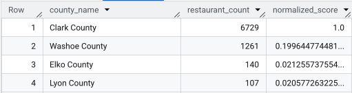
這張螢幕截圖顯示前 4 個正規化分數最高的郡。這個範例刻意省略了原始人口數。

縣級分析：找出最繁忙的商業區

現在我們已找出克拉克縣，下一步是放大畫面，找出商業活動最活躍的郵遞區號。根據現有咖啡店的資料，我們知道如果咖啡店位於主要品牌密集度高的區域，成效會比較好，因此我們會將此做為人潮眾多的指標。

這項查詢會使用 Places Insights 中的 brands 表格，其中包含特定品牌的相關資訊。您可以查詢這個表格，找出支援的品牌清單。首先，我們定義目標品牌清單，然後將這份清單與主要地點洞察資料集合併，計算克拉克郡各郵遞區號內有多少這類商店。

如要達到這個目標，最有效率的方法是採取兩步驟做法：

1. 首先，我們會執行快速的非地理空間彙整作業，計算每個郵遞區號內的品牌數量。
2. 接著，我們會將這些結果加入公開資料集，取得地圖界線以進行視覺化。

使用 postal_code_names 欄位計算品牌數量

第一個查詢會執行核心計數邏輯。這會篩選克拉克郡的地點，然後取消巢狀結構的 postal_code_names 陣列，依郵遞區號分組品牌數量。

WITH brand_names AS (
  -- First, select the chains we are interested in by name
  SELECT
    id,
    name
  FROM
    `places_insights___us.brands`
  WHERE
    name IN ('7-Eleven', 'CVS', 'Walgreens', 'Subway Restaurants', "McDonald's")
)
SELECT WITH AGGREGATION_THRESHOLD
  postal_code,
  COUNT(*) AS total_brand_count
FROM
  `places_insights___us.places` AS places_table,
  -- Unnest the built-in postal code and brand ID arrays
  UNNEST(places_table.postal_code_names) AS postal_code,
  UNNEST(places_table.brand_ids) AS brand_id
JOIN
  brand_names
  ON brand_names.id = brand_id
WHERE
  -- Filter directly on the administrative area fields in the places table
  places_table.administrative_area_level_2_name = 'Clark County'
  AND places_table.administrative_area_level_1_name = 'Nevada'
GROUP BY
  postal_code
ORDER BY
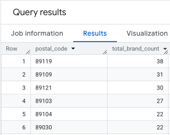
  total_brand_count DESC

輸出結果是郵遞區號和對應品牌數量的表格。

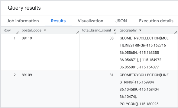
附加郵遞區號幾何圖形以供對應

現在我們有了計數，可以取得視覺化所需的 polygon 形狀。第二項查詢會採用第一項查詢，並將其包裝在名為 brand_counts_by_zip 的一般資料表運算式 (CTE) 中，然後將結果加入公開的 geo_us_boundaries.zip_codes table。這會將幾何圖形有效附加至預先計算的計數。

WITH brand_counts_by_zip AS (
  -- This will be the entire query from the previous step, without the final ORDER BY (excluded for brevity).
  . . .
)
-- Now, join the aggregated results to the boundaries table
SELECT
  counts.postal_code,
  counts.total_brand_count,
  -- Simplify the geometry for faster rendering in maps
  ST_SIMPLIFY(zip_boundaries.zip_code_geom, 100) AS geography
FROM
  brand_counts_by_zip AS counts
JOIN
  `bigquery-public-data.geo_us_boundaries.zip_codes` AS zip_boundaries
  ON counts.postal_code = zip_boundaries.zip_code
ORDER BY
  counts.total_brand_count DESC

輸出內容為郵遞區號表、對應的品牌數量，以及郵遞區號幾何圖形。

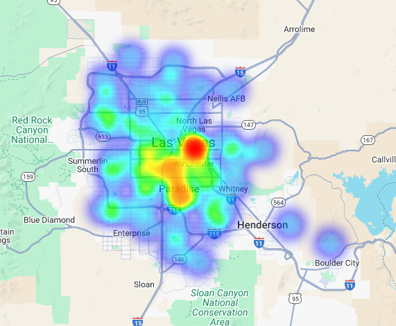
我們可以將這項資料視覺化為熱視圖。顏色越深的紅色區域代表目標品牌越密集，可協助我們找出拉斯維加斯商業最密集的區域。

超區域分析：為個別格線區域評分

找出拉斯維加斯的大概區域後，接下來就要進行細部分析。我們會在這一層加入特定的業務知識。我們知道，如果咖啡店附近有其他商家在尖峰時段 (例如上午稍晚和午餐時段) 也很忙碌，咖啡店的生意就會興隆。

下一個查詢會非常具體。首先，這項技術會使用標準 H3 地理空間索引 (解析度為 8)，在拉斯維加斯都會區建立細密的六邊形格線，以便在微觀層面分析該區域。查詢會先找出所有在尖峰時段 (週一上午 10 點至下午 2 點) 營業的互補商家。

接著，我們會為每個地點類型套用加權分數。對我們來說，附近的餐廳比便利商店更有價值，因此餐廳的乘數較高。這樣我們就能為每個小區域提供自訂 suitability_score。

這段摘錄內容著重於加權評分邏輯，其中會參照預先計算的營業時間檢查旗標 (is_open_monday_window)：

. . .
(
  COUNTIF('restaurant' IN UNNEST(types) AND is_open_monday_window) * 8 +
  COUNTIF('convenience_store' IN UNNEST(types) AND is_open_monday_window) * 3 +
  COUNTIF('bar' IN UNNEST(types) AND is_open_monday_window) * 7 +
  COUNTIF('tourist_attraction' IN UNNEST(types) AND is_open_monday_window) * 6 +
  COUNTIF('casino' IN UNNEST(types) AND is_open_monday_window) * 7
) AS suitability_score
. . .

展開完整查詢

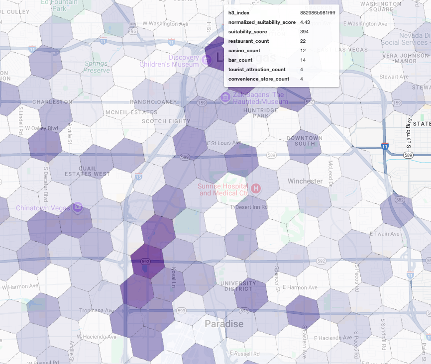
    -- This query calculates a custom 'suitability score' for different areas in the Las Vegas
-- metropolitan area to identify prime commercial zones. It uses a weighted model based
-- on the density of specific business types that are open during a target time window.

-- Step 1: Pre-filter the dataset to only include relevant places.
-- This CTE finds all places in our target localities (Las Vegas, Spring Valley, etc.) and
-- adds a boolean flag 'is_open_monday_window' for those open during the target time.
WITH PlacesInTargetAreaWithOpenFlag AS (
  SELECT
    point,
    types,
    EXISTS(
      SELECT 1
      FROM UNNEST(regular_opening_hours.monday) AS monday_hours
      WHERE
        monday_hours.start_time <= TIME '10:00:00'
        AND monday_hours.end_time >= TIME '14:00:00'
    ) AS is_open_monday_window
  FROM
    `places_insights___us.places`
  WHERE
    EXISTS (
        SELECT 1 FROM UNNEST(locality_names) AS locality
        WHERE locality IN ('Las Vegas', 'Spring Valley', 'Paradise', 'North Las Vegas', 'Winchester')
    )
    AND administrative_area_level_1_name = 'Nevada'
),
-- Step 2: Aggregate the filtered places into H3 cells and calculate the suitability score.
-- Each place's location is converted to an H3 index (at resolution 8). The query then
-- calculates a weighted 'suitability_score' and individual counts for each business type
-- within that cell.
TileScores AS (
  SELECT WITH AGGREGATION_THRESHOLD
    -- Convert each place's geographic point into an H3 cell index.
    `carto-os.carto.H3_FROMGEOGPOINT`(point, 8) AS h3_index,

    -- Calculate the weighted score based on the count of places of each type
    -- that are open during the target window.
    (
      COUNTIF('restaurant' IN UNNEST(types) AND is_open_monday_window) * 8 +
      COUNTIF('convenience_store' IN UNNEST(types) AND is_open_monday_window) * 3 +
      COUNTIF('bar' IN UNNEST(types) AND is_open_monday_window) * 7 +
      COUNTIF('tourist_attraction' IN UNNEST(types) AND is_open_monday_window) * 6 +
      COUNTIF('casino' IN UNNEST(types) AND is_open_monday_window) * 7
    ) AS suitability_score,

    -- Also return the individual counts for each category for detailed analysis.
    COUNTIF('restaurant' IN UNNEST(types) AND is_open_monday_window) AS restaurant_count,
    COUNTIF('convenience_store' IN UNNEST(types) AND is_open_monday_window) AS convenience_store_count,
    COUNTIF('bar' IN UNNEST(types) AND is_open_monday_window) AS bar_count,
    COUNTIF('tourist_attraction' IN UNNEST(types) AND is_open_monday_window) AS tourist_attraction_count,
    COUNTIF('casino' IN UNNEST(types) AND is_open_monday_window) AS casino_count
  FROM
    -- CHANGED: This now references the CTE with the expanded area.
    PlacesInTargetAreaWithOpenFlag
  -- Group by the H3 index to ensure all calculations are per-cell.
  GROUP BY
    h3_index
),
-- Step 3: Find the maximum suitability score across all cells.
-- This value is used in the next step to normalize the scores to a consistent scale (e.g., 0-10).
MaxScore AS (
  SELECT MAX(suitability_score) AS max_score FROM TileScores
)
-- Step 4: Assemble the final results.
-- This joins the scored tiles with the max score, calculates the normalized score,
-- generates the H3 cell's polygon geometry for mapping, and orders the results.
SELECT
  ts.h3_index,
  -- Generate the hexagonal polygon for the H3 cell for visualization.
  `carto-os.carto.H3_BOUNDARY`(ts.h3_index) AS h3_geography,
  ts.restaurant_count,
  ts.convenience_store_count,
  ts.bar_count,
  ts.tourist_attraction_count,
  ts.casino_count,
  ts.suitability_score,
  -- Normalize the score to a 0-10 scale for easier interpretation.
  ROUND(
    CASE
      WHEN ms.max_score = 0 THEN 0
      ELSE (ts.suitability_score / ms.max_score) * 10
    END,
    2
  ) AS normalized_suitability_score
FROM
  -- A cross join is efficient here as MaxScore contains only one row.
  TileScores ts, MaxScore ms
-- Display the highest-scoring locations first.
ORDER BY
  normalized_suitability_score DESC;
    

在地圖上顯示這些分數，即可清楚看出哪些地點最適合開店。深紫色方塊主要位於拉斯維加斯大道和市中心附近，是我們新咖啡廳最有潛力的區域。

競品分析：找出現有咖啡廳

我們的適當性模型已成功找出最有希望的區域，但高分並不保證一定能成功。現在我們必須將這項資料與競爭對手資料重疊。理想地點是現有咖啡店密度較低的潛力區域，因為我們希望找到明顯的市場缺口。

為此，我們會使用 PLACES_COUNT_PER_H3 函式。這個函式的設計宗旨，是有效率地依 H3 儲存格，傳回指定地理區域內的地點數量。

首先，我們會動態定義整個拉斯維加斯都會區的地理位置。 我們不會只依賴單一地區，而是查詢公開的 Overture 地圖資料集，取得拉斯維加斯及其周圍主要地區的邊界，並使用 ST_UNION_AGG 將這些邊界合併為單一多邊形。接著，我們會將這個區域傳遞至函式，要求函式計算所有營業中的咖啡館。

這項查詢會定義都會區，並呼叫函式來取得 H3 儲存格中的咖啡廳數量：

-- Define a variable to hold the combined geography for the Las Vegas metro area.
DECLARE las_vegas_metro_area GEOGRAPHY;

-- Set the variable by fetching the shapes for the five localities from Overture Maps
-- and merging them into a single polygon using ST_UNION_AGG.
SET las_vegas_metro_area = (
  SELECT
    ST_UNION_AGG(geometry)
  FROM
    `bigquery-public-data.overture_maps.division_area`
  WHERE
    country = 'US'
    AND region = 'US-NV'
    AND names.primary IN ('Las Vegas', 'Spring Valley', 'Paradise', 'North Las Vegas', 'Winchester')
);

-- Call the PLACES_COUNT_PER_H3 function with our defined area and parameters.
SELECT
  *
FROM
  `places_insights___us.PLACES_COUNT_PER_H3`(
    JSON_OBJECT(
      -- Use the metro area geography we just created.
      'geography', las_vegas_metro_area,
      -- Specify 'coffee_shop' as the place type to count.
      'types', ["coffee_shop"],
      -- Best practice: Only count places that are currently operational.
      'business_status', ['OPERATIONAL'],
      -- Set the H3 grid resolution to 8.
      'h3_resolution', 8
    )
  );

函式會傳回表格，其中包含 H3 儲存格索引、幾何圖形、咖啡店總數，以及咖啡店的 Place ID 樣本：

雖然匯總計數很有用，但查看實際競爭對手至關重要。 我們將在此階段從 Places 洞察資料集轉換至 Places API。從正規化合適度分數最高的儲存格中擷取 sample_place_ids，即可呼叫 Place Details API，擷取每個競爭對手的詳細資料，例如名稱、地址、評分和位置。

這需要比較先前查詢 (產生適用性分數) 和 PLACES_COUNT_PER_H3 查詢的結果。您可以使用 H3 儲存格索引，從正規化適用性分數最高的儲存格取得咖啡店數量和 ID。

這段 Python 程式碼示範如何執行這項比較。

    # Isolate the Top 5 Most Suitable H3 Cells
    top_suitability_cells = gdf_suitability.head(5)

    # Extract the 'h3_index' values from these top 5 cells into a list.
    top_h3_indexes = top_suitability_cells['h3_index'].tolist()
    print(f"The top 5 H3 indexes are: {top_h3_indexes}")

    # Now, we find the rows in our DataFrame where the
    # 'h3_cell_index' matches one of the indexes from our top 5 list.

    coffee_counts_in_top_zones = gdf_coffee_shops[
        gdf_coffee_shops['h3_cell_index'].isin(top_h3_indexes)
    ]

現在我們已取得 H3 儲存格中現有咖啡店的地點 ID 清單，這些儲存格的適用性分數最高，因此可以要求取得每個地點的詳細資料。

如要執行這項操作，您可以針對每個地點 ID 直接向 Place Details API 傳送要求，也可以使用用戶端程式庫執行呼叫。請記得設定 FieldMask 參數，只要求所需的資料。

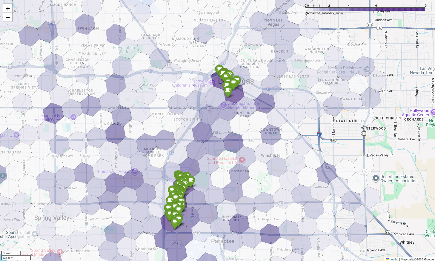
最後，我們將所有內容整合為單一的強大視覺化效果。我們以紫色適宜性等值線地圖做為基礎圖層，然後為從 Places API 擷取的每間咖啡店新增圖釘。這張最終地圖會整合所有分析結果，讓您一目瞭然：深紫色區域顯示潛力，綠色圖釘則顯示目前市場的實際情況。

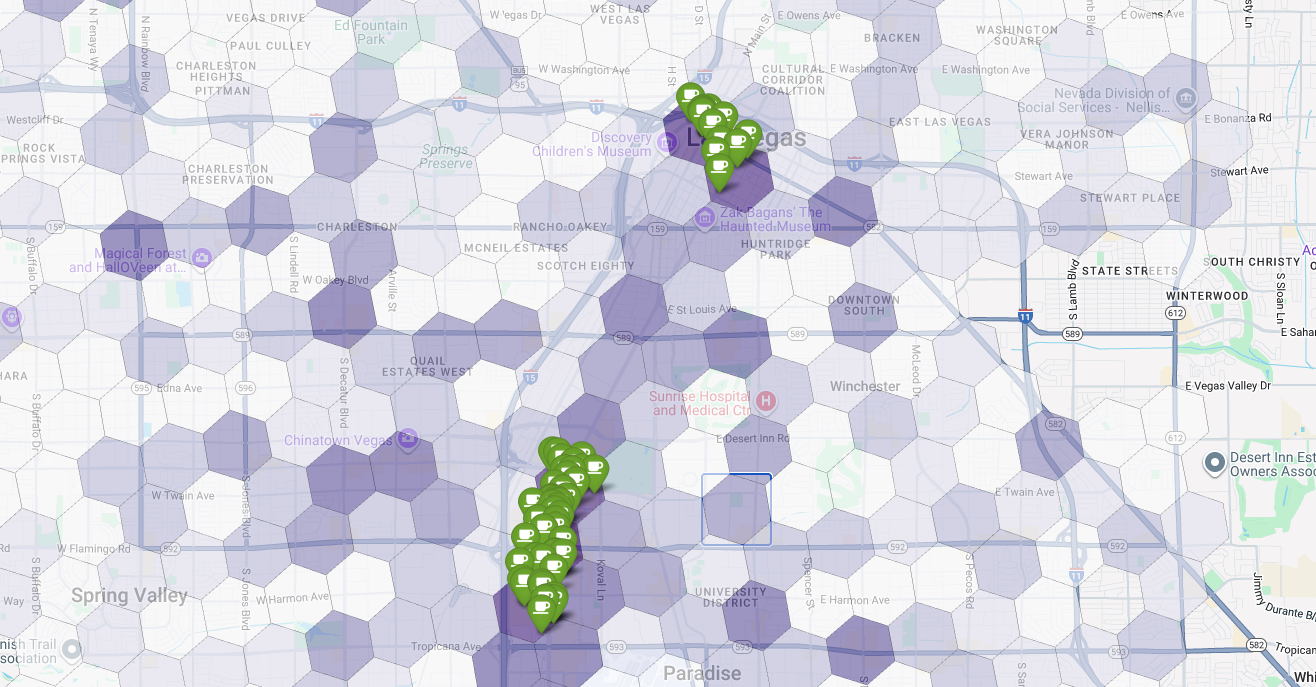
只要找出沒有或只有少量圖釘的深紫色儲存格，就能準確找出最適合新地點的區域。

上述兩個儲存格的適用性分數很高，但仍有一些明顯的差距，可能適合做為新咖啡店的地點。

結論

在本文件中，我們從全州範圍的問題「要在哪裡擴展？」，轉向以資料為依據的當地答案。只要疊加不同的資料集並套用自訂的業務邏輯，就能有系統地降低重大業務決策的相關風險。這個工作流程結合了 BigQuery 的規模、地點洞察的豐富性，以及 Places API 的即時詳細資料，為任何想運用位置情報實現策略性成長的機構提供強大的範本。

後續步驟

• 請根據您的業務邏輯、目標地理區域和專有資料集，調整這個工作流程。
• 探索 Places Insights 資料集中的其他資料欄位，例如評論數、價格等級和使用者評分，進一步豐富模型。
• 自動執行這項程序，建立內部網站選取資訊主頁，用於動態評估新市場。

深入瞭解說明文件：

• 地點洞察總覽
• 地點洞察函式
• BigQuery 地理空間分析
• Places API

貢獻者

Henrik Valve | DevX 工程師