使用 Places Insights 和 BigQuery 执行选址

简介

本文档介绍了如何通过组合使用地点数据分析数据集、BigQuery 中的公共地理空间数据和地点详情 API来构建选址解决方案。

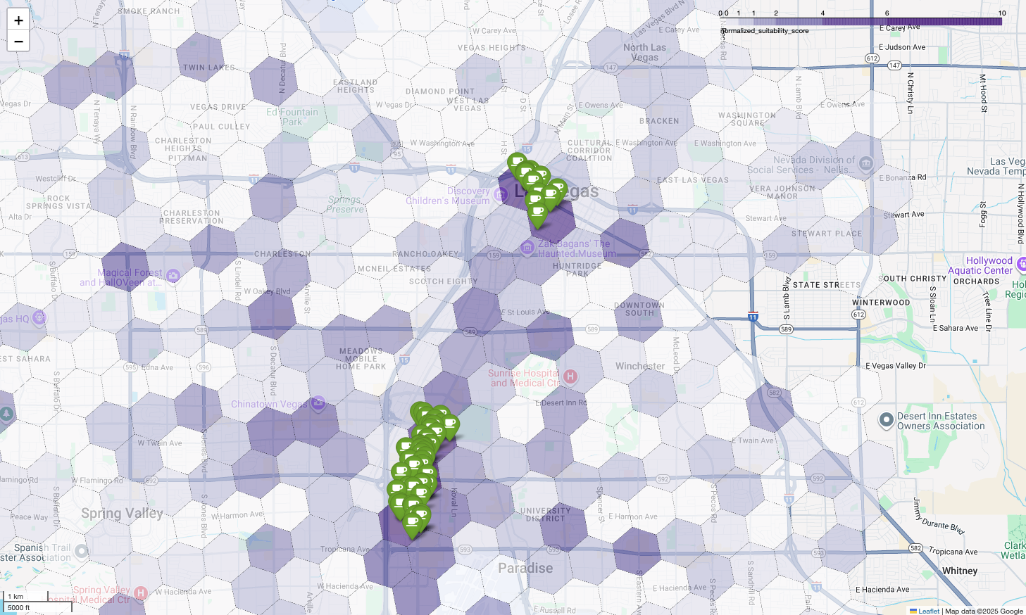
拉斯维加斯地图，显示了潜在的新咖啡店位置，其中紫色数据覆盖表示潜在的新咖啡店位置，绿色图钉表示现有竞争对手的位置。

上图展示了 Google Cloud Next 2025 上演示的输出，您可以在YouTube上观看该演示。您可以使用示例笔记本运行用于生成这些结果的代码。

在 Google Colab 中运行

在 GitHub 上查看源代码

业务挑战

假设您拥有一家成功的连锁咖啡店，并希望扩展到内华达州等您尚未涉足的新州。开设新店是一项重大投资，做出数据驱动型决策对于成功至关重要。您应该从何处入手？

本指南将引导您完成多层分析，以找出新咖啡店的最佳位置。我们将从全州范围的视角开始，逐步将搜索范围缩小到特定县和商业区域，最后执行超本地化分析，通过绘制竞争对手分布图来为各个区域打分并找出市场空白。

解决方案工作流

此过程遵循逻辑漏斗，从广阔的范围开始，逐步细化，以缩小搜索范围并提高对最终选址的信心。

前提条件和环境设置

在深入分析之前，您需要一个具有一些关键功能的环境。虽然本指南将介绍使用 SQL 和 Python 的实现，但一般原则可以应用于其他技术堆栈。

作为前提条件，请确保您的环境可以：

在 BigQuery 中执行查询。
访问地点数据分析，如需了解详情，请参阅设置地点数据分析
订阅 bigquery-public-data 和美国人口普查局县人口总数中的公共数据集

您还需要能够在地图上直观呈现地理空间数据，这对于解读每个分析步骤的结果至关重要。有很多方法可以实现这一点。您可以使用直接连接到 BigQuery 的 Looker Studio 等 BI 工具，也可以使用 Python 等数据科学语言。

州级分析：找出最佳县

我们的第一步是进行广泛的分析，以找出内华达州最有前景的县。我们将“有前景”定义为人口众多且现有餐厅密度高，这表明当地的餐饮文化浓厚。

我们的 BigQuery 查询通过利用地点数据分析数据集中提供的内置地址组件来实现这一点。该查询首先使用 administrative_area_level_1_name 字段过滤数据，以仅包含内华达州境内的地点，然后统计餐厅数量。然后，它进一步细化此集合，以仅包含类型数组包含“restaurant”的地点。最后，它按县名 (administrative_area_level_2_name) 对这些结果进行分组，以生成每个县的计数。此方法利用了数据集的内置预编索引地址结构。

此摘录展示了如何将县几何图形与地点数据分析联接，并针对特定地点类型（restaurant）进行过滤：

SELECT WITH AGGREGATION_THRESHOLD
  administrative_area_level_2_name,
  COUNT(*) AS restaurant_count
FROM
  `places_insights___us.places`
WHERE
  -- Filter for the state of Nevada
  administrative_area_level_1_name = 'Nevada'
  -- Filter for places that are restaurants
  AND 'restaurant' IN UNNEST(types)
  -- Filter for operational places only
  AND business_status = 'OPERATIONAL'
  -- Exclude rows where the county name is null
  AND administrative_area_level_2_name IS NOT NULL
GROUP BY
  administrative_area_level_2_name
ORDER BY
  restaurant_count DESC

仅统计餐厅数量是不够的；我们需要将其与人口数据进行平衡，才能真正了解市场饱和度和机会。我们将使用美国人口普查局县人口总数中的人口数据。

为了比较这两个截然不同的指标（地点计数与庞大的人口数量），我们使用最小-最大归一化。此技术将这两个指标都缩放到一个通用范围（0 到 1）。然后，我们将它们合并为一个 normalized_score，为每个指标赋予 50% 的权重，以便进行平衡比较。

此摘录展示了计算得分的核心逻辑。它结合了归一化的人口和餐厅数量：

(
    -- Normalize restaurant count (scales to a 0-1 value) and apply 50% weight
    SAFE_DIVIDE(restaurant_count - min_restaurants, max_restaurants - min_restaurants) * 0.5
    +
    -- Normalize population (scales to a 0-1 value) and apply 50% weight
    SAFE_DIVIDE(population_2023 - min_pop, max_pop - min_pop) * 0.5
  ) AS normalized_score

运行完整查询后，系统会返回县列表、餐厅数量、人口和归一化得分。按 normalized_score DESC 排序会显示克拉克县是明显的胜出者，值得进一步调查，是头号竞争者。

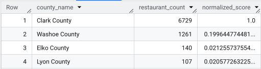
此屏幕截图显示了按归一化得分排名的前 4 个县。此示例中有意省略了原始人口计数。

县级分析：找出最繁忙的商业区

现在我们已经确定了克拉克县，下一步是放大以找出商业活动最频繁的邮政编码。根据我们现有咖啡店的数据，我们知道，如果咖啡店位于主要品牌密度较高的区域附近，业绩会更好，因此我们将此作为实体店客流量高的代理。

此查询使用地点数据分析中的 brands 表，其中包含有关特定品牌的信息。您可以查询此表以发现受支持的品牌列表。我们首先定义目标品牌列表，然后将其与主要的地点数据分析数据集联接，以统计克拉克县中每个邮政编码内有多少家指定商店。

实现此目标的最有效方法是采用两步法：

首先，我们将执行快速的非地理空间汇总，以统计每个邮政编码内的品牌数量。
其次，我们将这些结果与公共数据集联接，以获取地图边界以进行可视化。

使用 `postal_code_names` 字段统计品牌数量

第一个查询执行核心计数逻辑。它会过滤克拉克县的地点，然后取消嵌套 postal_code_names 数组，以按邮政编码对品牌计数进行分组。

WITH brand_names AS (
  -- First, select the chains we are interested in by name
  SELECT
    id,
    name
  FROM
    `places_insights___us.brands`
  WHERE
    name IN ('7-Eleven', 'CVS', 'Walgreens', 'Subway Restaurants', "McDonald's")
)
SELECT WITH AGGREGATION_THRESHOLD
  postal_code,
  COUNT(*) AS total_brand_count
FROM
  `places_insights___us.places` AS places_table,
  -- Unnest the built-in postal code and brand ID arrays
  UNNEST(places_table.postal_code_names) AS postal_code,
  UNNEST(places_table.brand_ids) AS brand_id
JOIN
  brand_names
  ON brand_names.id = brand_id
WHERE
  -- Filter directly on the administrative area fields in the places table
  places_table.administrative_area_level_2_name = 'Clark County'
  AND places_table.administrative_area_level_1_name = 'Nevada'
GROUP BY
  postal_code
ORDER BY
  total_brand_count DESC

输出是一个包含邮政编码及其相应品牌计数的表格。

一个列出邮政编码及其品牌总数的查询结果表，其中 89119 的品牌总数最高，为 38。

附加邮政编码几何图形以进行地图绘制

现在我们有了计数，就可以获取可视化所需的多边形形状。第二个查询会获取我们的第一个查询，将其封装在名为 brand_counts_by_zip 的通用表表达式 (CTE) 中，并将其结果与公共 geo_us_boundaries.zip_codes table 联接。这样可以高效地将几何图形附加到我们预先计算的计数中。

WITH brand_counts_by_zip AS (
  -- This will be the entire query from the previous step, without the final ORDER BY (excluded for brevity).
  . . .
)
-- Now, join the aggregated results to the boundaries table
SELECT
  counts.postal_code,
  counts.total_brand_count,
  -- Simplify the geometry for faster rendering in maps
  ST_SIMPLIFY(zip_boundaries.zip_code_geom, 100) AS geography
FROM
  brand_counts_by_zip AS counts
JOIN
  `bigquery-public-data.geo_us_boundaries.zip_codes` AS zip_boundaries
  ON counts.postal_code = zip_boundaries.zip_code
ORDER BY
  counts.total_brand_count DESC

输出是一个包含邮政编码、相应品牌计数和邮政编码几何图形的表格。

查询结果表，其中包含邮政编码、品牌数量以及用于可视化的相应地理多边形数据。

我们可以将此数据可视化为热图。颜色较深的红色区域表示目标品牌的集中度较高，这表明拉斯维加斯商业密度最高的区域。

一张显示拉斯维加斯目标品牌集中度的热图，其中红色和黄色表示集中度最高。

超本地化分析：为各个网格区域评分

确定拉斯维加斯的大致区域后，接下来需要进行精细分析。在此阶段，我们将融入特定的业务知识。我们知道，一家优秀的咖啡店在其他商家（例如上午晚些时候和午餐时段）繁忙时，也会生意兴隆。

我们的下一个查询将非常具体。它首先使用标准 H3 地理空间索引（分辨率为 8）在拉斯维加斯大都会区创建一个精细的六边形网格，以便在微观层面分析该区域。该查询首先找出在我们的高峰时段（周一上午 10 点至下午 2 点）营业的所有互补商家。

然后，我们为每种地点类型应用加权得分。附近的餐厅比便利店对我们更有价值，因此餐厅的乘数更高。这样，我们就可以为每个小区域获得自定义的 suitability_score。

此摘录突出显示了加权评分逻辑，该逻辑引用了预先计算的标志 (is_open_monday_window) 以检查营业时间：

. . .
(
  COUNTIF('restaurant' IN UNNEST(types) AND is_open_monday_window) * 8 +
  COUNTIF('convenience_store' IN UNNEST(types) AND is_open_monday_window) * 3 +
  COUNTIF('bar' IN UNNEST(types) AND is_open_monday_window) * 7 +
  COUNTIF('tourist_attraction' IN UNNEST(types) AND is_open_monday_window) * 6 +
  COUNTIF('casino' IN UNNEST(types) AND is_open_monday_window) * 7
) AS suitability_score
. . .

展开即可查看完整查询

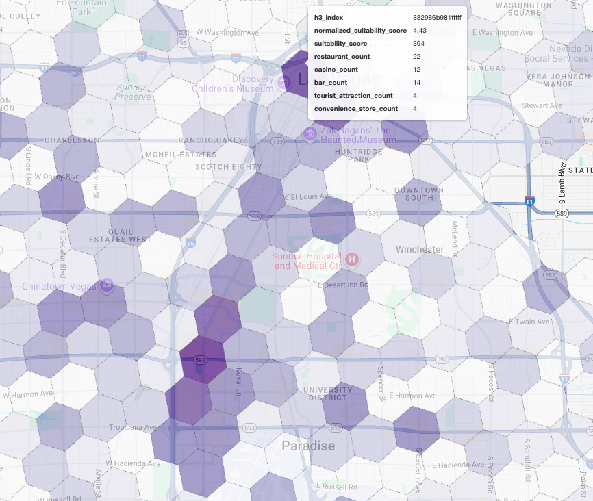
    -- This query calculates a custom 'suitability score' for different areas in the Las Vegas
-- metropolitan area to identify prime commercial zones. It uses a weighted model based
-- on the density of specific business types that are open during a target time window.

-- Step 1: Pre-filter the dataset to only include relevant places.
-- This CTE finds all places in our target localities (Las Vegas, Spring Valley, etc.) and
-- adds a boolean flag 'is_open_monday_window' for those open during the target time.
WITH PlacesInTargetAreaWithOpenFlag AS (
  SELECT
    point,
    types,
    EXISTS(
      SELECT 1
      FROM UNNEST(regular_opening_hours.monday) AS monday_hours
      WHERE
        monday_hours.start_time <= TIME '10:00:00'
        AND monday_hours.end_time >= TIME '14:00:00'
    ) AS is_open_monday_window
  FROM
    `places_insights___us.places`
  WHERE
    EXISTS (
        SELECT 1 FROM UNNEST(locality_names) AS locality
        WHERE locality IN ('Las Vegas', 'Spring Valley', 'Paradise', 'North Las Vegas', 'Winchester')
    )
    AND administrative_area_level_1_name = 'Nevada'
),
-- Step 2: Aggregate the filtered places into H3 cells and calculate the suitability score.
-- Each place's location is converted to an H3 index (at resolution 8). The query then
-- calculates a weighted 'suitability_score' and individual counts for each business type
-- within that cell.
TileScores AS (
  SELECT WITH AGGREGATION_THRESHOLD
    -- Convert each place's geographic point into an H3 cell index.
    `carto-os.carto.H3_FROMGEOGPOINT`(point, 8) AS h3_index,

    -- Calculate the weighted score based on the count of places of each type
    -- that are open during the target window.
    (
      COUNTIF('restaurant' IN UNNEST(types) AND is_open_monday_window) * 8 +
      COUNTIF('convenience_store' IN UNNEST(types) AND is_open_monday_window) * 3 +
      COUNTIF('bar' IN UNNEST(types) AND is_open_monday_window) * 7 +
      COUNTIF('tourist_attraction' IN UNNEST(types) AND is_open_monday_window) * 6 +
      COUNTIF('casino' IN UNNEST(types) AND is_open_monday_window) * 7
    ) AS suitability_score,

    -- Also return the individual counts for each category for detailed analysis.
    COUNTIF('restaurant' IN UNNEST(types) AND is_open_monday_window) AS restaurant_count,
    COUNTIF('convenience_store' IN UNNEST(types) AND is_open_monday_window) AS convenience_store_count,
    COUNTIF('bar' IN UNNEST(types) AND is_open_monday_window) AS bar_count,
    COUNTIF('tourist_attraction' IN UNNEST(types) AND is_open_monday_window) AS tourist_attraction_count,
    COUNTIF('casino' IN UNNEST(types) AND is_open_monday_window) AS casino_count
  FROM
    -- CHANGED: This now references the CTE with the expanded area.
    PlacesInTargetAreaWithOpenFlag
  -- Group by the H3 index to ensure all calculations are per-cell.
  GROUP BY
    h3_index
),
-- Step 3: Find the maximum suitability score across all cells.
-- This value is used in the next step to normalize the scores to a consistent scale (e.g., 0-10).
MaxScore AS (
  SELECT MAX(suitability_score) AS max_score FROM TileScores
)
-- Step 4: Assemble the final results.
-- This joins the scored tiles with the max score, calculates the normalized score,
-- generates the H3 cell's polygon geometry for mapping, and orders the results.
SELECT
  ts.h3_index,
  -- Generate the hexagonal polygon for the H3 cell for visualization.
  `carto-os.carto.H3_BOUNDARY`(ts.h3_index) AS h3_geography,
  ts.restaurant_count,
  ts.convenience_store_count,
  ts.bar_count,
  ts.tourist_attraction_count,
  ts.casino_count,
  ts.suitability_score,
  -- Normalize the score to a 0-10 scale for easier interpretation.
  ROUND(
    CASE
      WHEN ms.max_score = 0 THEN 0
      ELSE (ts.suitability_score / ms.max_score) * 10
    END,
    2
  ) AS normalized_suitability_score
FROM
  -- A cross join is efficient here as MaxScore contains only one row.
  TileScores ts, MaxScore ms
-- Display the highest-scoring locations first.
ORDER BY
  normalized_suitability_score DESC;

在地图上直观呈现这些得分会显示明显的胜出地点。颜色最深的紫色图块（主要位于拉斯维加斯大道和市中心附近）是新咖啡店最具潜力的区域。

一张拉斯维加斯分级统计图，使用紫色六边形网格显示适宜性得分，颜色越深表示潜力越大。

竞争对手分析：找出现有咖啡店

我们的适宜性模型已成功找出最有前景的区域，但仅凭高分并不能保证成功。我们现在必须将此与竞争对手数据叠加。理想的地点是现有咖啡店密度较低的高潜力区域，因为我们正在寻找明显的市场空白。

为此，我们使用 PLACES_COUNT_PER_H3 函数。此函数旨在高效地按 H3 单元格返回指定地理区域内的地点计数。

首先，我们动态定义整个拉斯维加斯都市圈的地理区域。我们不依赖于单个市行政区，而是查询公共 Overture Maps 数据集以获取拉斯维加斯及其周边主要市行政区的边界，并使用 ST_UNION_AGG 将它们合并为一个多边形。然后，我们将此区域传递给该函数，要求它统计所有营业的咖啡店。

此查询定义了大都会区，并调用该函数以获取 H3 单元格中的咖啡店计数：

-- Define a variable to hold the combined geography for the Las Vegas metro area.
DECLARE las_vegas_metro_area GEOGRAPHY;

-- Set the variable by fetching the shapes for the five localities from Overture Maps
-- and merging them into a single polygon using ST_UNION_AGG.
SET las_vegas_metro_area = (
  SELECT
    ST_UNION_AGG(geometry)
  FROM
    `bigquery-public-data.overture_maps.division_area`
  WHERE
    country = 'US'
    AND region = 'US-NV'
    AND names.primary IN ('Las Vegas', 'Spring Valley', 'Paradise', 'North Las Vegas', 'Winchester')
);

-- Call the PLACES_COUNT_PER_H3 function with our defined area and parameters.
SELECT
  *
FROM
  `places_insights___us.PLACES_COUNT_PER_H3`(
    JSON_OBJECT(
      -- Use the metro area geography we just created.
      'geography', las_vegas_metro_area,
      -- Specify 'coffee_shop' as the place type to count.
      'types', ["coffee_shop"],
      -- Best practice: Only count places that are currently operational.
      'business_status', ['OPERATIONAL'],
      -- Set the H3 grid resolution to 8.
      'h3_resolution', 8
    )
  );

该函数返回一个表格，其中包含 H3 单元格索引、其几何图形、咖啡店总数以及一些咖啡店的地点 ID 示例：

查询结果表，显示了 H3 单元格及其咖啡店数量和相应的示例地点 ID。

虽然汇总计数很有用，但了解实际的竞争对手至关重要。在此阶段，我们将从地点数据分析数据集过渡到 Places API。通过从归一化适宜性得分最高的单元格中提取 sample_place_ids，我们可以调用地点详情 API 来检索每个竞争对手的丰富详细信息，例如名称、地址、评分和位置。

这需要比较之前生成适宜性得分的查询的结果与 PLACES_COUNT_PER_H3 查询的结果。H3 单元格索引可用于从归一化适宜性得分最高的单元格中获取咖啡店计数和 ID。

以下 Python 代码演示了如何执行此比较。

    # Isolate the Top 5 Most Suitable H3 Cells
    top_suitability_cells = gdf_suitability.head(5)

    # Extract the 'h3_index' values from these top 5 cells into a list.
    top_h3_indexes = top_suitability_cells['h3_index'].tolist()
    print(f"The top 5 H3 indexes are: {top_h3_indexes}")

    # Now, we find the rows in our DataFrame where the
    # 'h3_cell_index' matches one of the indexes from our top 5 list.

    coffee_counts_in_top_zones = gdf_coffee_shops[
        gdf_coffee_shops['h3_cell_index'].isin(top_h3_indexes)
    ]

现在我们有了适宜性得分最高的 H3 单元格中已有的咖啡店的地点 ID 列表，可以请求有关每个地点的更多详细信息。

为此，您可以直接为每个地点 ID 向地点详情 API 发送请求，也可以使用客户端库执行调用。请务必设置 FieldMask 参数，以仅请求所需的数据。

最后，我们将所有内容合并为一个强大的可视化效果。我们将紫色适宜性分级统计图绘制为基础层，然后为从 Places API 检索到的每家咖啡店添加图钉。此最终地图提供了一个一目了然的视图，综合了我们的整个分析：深紫色区域显示了潜力，绿色图钉显示了当前市场的实际情况。

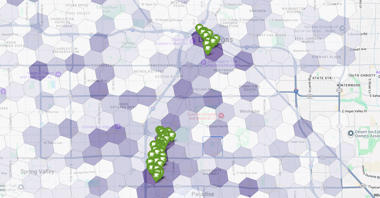
拉斯维加斯地图，其中显示了紫色六边形网格（表示高潜力区域）和绿色图钉（表示现有咖啡店）。

通过查找图钉很少或没有图钉的深紫色单元格，我们可以自信地找出最适合开设新店的确切区域。

一张拉斯维加斯两个高潜力紫色区域的近距离地图，显示了竞争对手的位置和明显的市场空白。

上述两个单元格的适宜性得分很高，但存在一些明显的空白，这些空白可能是开设新咖啡店的潜在地点。

总结

在本文档中，我们从“在哪里扩张？”这一全州范围的问题入手，最终得出了有数据支持的本地化答案。通过叠加不同的数据集并应用自定义业务逻辑，您可以系统地降低与重大业务决策相关的风险。此工作流结合了 BigQuery 的规模、地点数据分析的丰富性和 Places API 的实时详细信息，为任何希望使用地理位置智能来实现战略增长的组织提供了一个强大的模板。

后续步骤

根据您自己的业务逻辑、目标地理区域和专有数据集调整此工作流。
探索地点数据分析数据集中的其他数据字段，例如评价数量、价格水平和用户评分，以进一步丰富您的模型。
自动执行此过程，以创建一个内部选址信息中心，该信息中心可用于动态评估新市场。

深入了解文档：

贡献者

Henrik Valve | DevX 工程师