Logistic regression: Calculating a probability with the sigmoid function

Many problems require a probability estimate as output. Logistic regression is an extremely efficient mechanism for calculating probabilities. Practically speaking, you can use the returned probability in either of the following two ways:

• Applied "as is." For example, if a spam-prediction model takes an email as input and outputs a value of 0.932, this implies a 93.2% probability that the email is spam.

• Converted to a binary category such as True or False, Spam or Not Spam.

This module focuses on using logistic regression model output as-is. In the Classification module, you'll learn how to convert this output into a binary category.

Sigmoid function

You might be wondering how a logistic regression model can ensure its output represents a probability, always outputting a value between 0 and 1. As it happens, there's a family of functions called logistic functions whose output has those same characteristics. The standard logistic function, also known as the sigmoid function (sigmoid means "s-shaped"), has the formula:

\[f(x) = \frac{1}{1 + e^{-x}}\]

Figure 1 shows the corresponding graph of the sigmoid function.

Figure 1. Graph of the sigmoid function. The curve approaches 0 as x values decrease to negative infinity, and 1 as x values increase toward infinity.

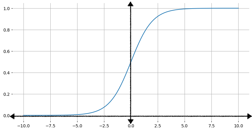
As the input, x, increases, the output of the sigmoid function approaches but never reaches 1. Similarly, as the input decreases, the sigmoid function's output approaches but never reaches 0.

Click here for a deeper dive into the math behind the sigmoid function

The table below shows the output values of the sigmoid function for input values in the range –7 to 7. Note how quickly the sigmoid approaches 0 for decreasing negative input values, and how quickly the sigmoid approaches 1 for increasing positive input values.

However, no matter how large or how small the input value, the output will always be greater than 0 and less than 1.

Input	Sigmoid output
-7	0.001
-6	0.002
-5	0.007
-4	0.018
-3	0.047
-2	0.119
-1	0.269
0	0.50
1	0.731
2	0.881
3	0.952
4	0.982
5	0.993
6	0.997
7	0.999

Transforming linear output using the sigmoid function

The following equation represents the linear component of a logistic regression model:

\[z = b + w_1x_1 + w_2x_2 + \ldots + w_Nx_N\]

where:

• z is the output of the linear equation, also called the log odds.
• b is the bias.
• The w values are the model's learned weights.
• The x values are the feature values for a particular example.

To obtain the logistic regression prediction, the z value is then passed to the sigmoid function, yielding a value (a probability) between 0 and 1:

\[y' = \frac{1}{1 + e^{-z}}\]

where:

• y' is the output of the logistic regression model.
• z is the linear output (as calculated in the preceding equation).

Click here to learn more about log-odds

In the equation $z = b + w_1x_1 + w_2x_2 + \ldots + w_Nx_N$, z is referred to as the log-odds because if you start with the following sigmoid function (where $y$ is the output of a logistic regression model, representing a probability):

$$y = \frac{1}{1 + e^{-z}}$$

And then solve for z:

$$ z = \log\left(\frac{y}{1-y}\right) $$

Then z is defined as the log of the ratio of the probabilities of the two possible outcomes: y and 1 – y.

Figure 2 illustrates how linear output is transformed to logistic regression output using these calculations.

Figure 2. Left: graph of the linear function z = 2x + 5, with three points highlighted. Right: Sigmoid curve with the same three points highlighted after being transformed by the sigmoid function.

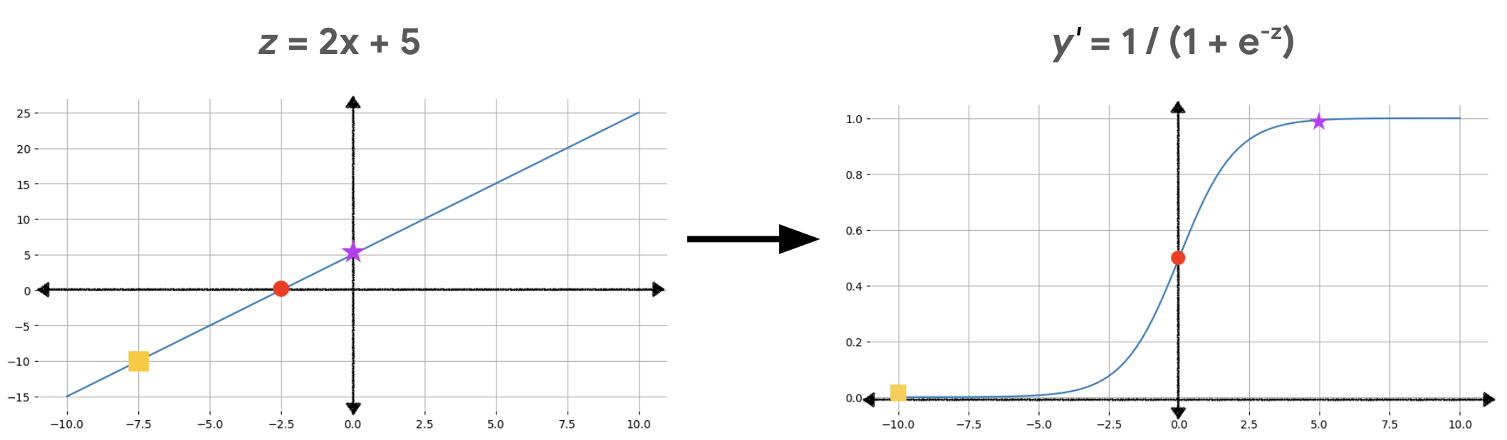
In Figure 2, a linear equation becomes input to the sigmoid function, which bends the straight line into an s-shape. Notice that the linear equation can output very big or very small values of z, but the output of the sigmoid function, y', is always between 0 and 1, exclusive. For example, the orange rectangle on the left graph has a z value of -10, but the sigmoid function in the right graph maps that -10 into a y' value of 0.00004.

Exercise: Check your understanding

A logistic regression model with three features has the following bias and weights:

\[\begin{align} b &= 1 \\ w_1 &= 2 \\ w_2 &= -1 \\ w_3 &= 5 \end{align} \]

Given the following input values:

\[\begin{align} x_1 &= 0 \\ x_2 &= 10 \\ x_3 &= 2 \end{align} \]

Answer the following two questions.

1. What is the value of z for these input values?

–1

0

0.731

1

Correct! The linear equation defined by the weights and bias is z = 1 + 2x₁ – x₂ + 5 x₃. Plugging the input values into the equation produces z = 1 + (2)(0) - (10) + (5)(2) = 1

2. What is the logistic regression prediction for these input values?

0.268

0.5

0.731

As calculated in #1 above, the log-odds for the input values is 1. Plugging that value for z into the sigmoid function:

\(y = \frac{1}{1 + e^{-z}} = \frac{1}{1 + e^{-1}} = \frac{1}{1 + 0.367} = \frac{1}{1.367} = 0.731\)

1

Remember, the output of the sigmoid function will always be greater than 0 and less than 1.

Key terms:

• Binary classification
• Log odds
• Logistic regression
• Sigmoid function