
코딩 수준: 초급
시간: 5분
프로젝트 유형: 커스텀 함수
목표
- 솔루션의 기능을 이해합니다.
- 솔루션 내에서 Apps Script 서비스의 기능을 이해합니다.
- 스크립트를 설정합니다.
- 스크립트를 실행합니다.
이 솔루션 정보
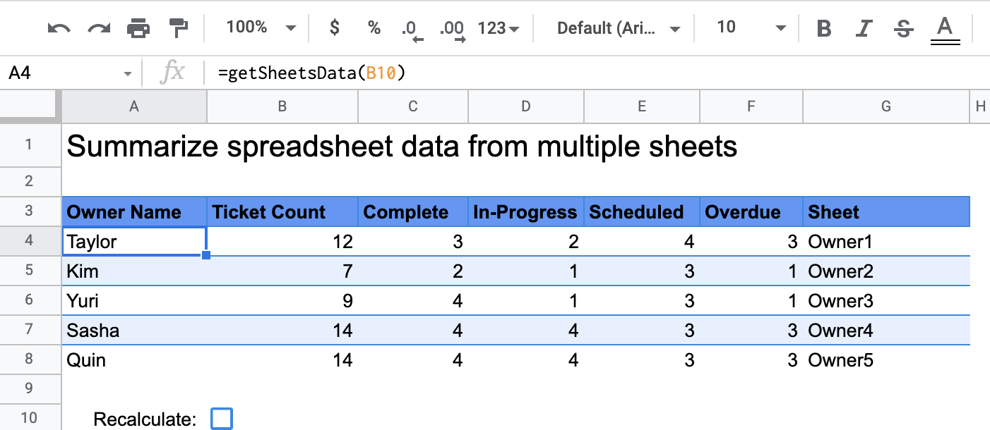
스프레드시트의 여러 시트에 유사한 구조화된 데이터(여러 팀원의 고객 지원 측정항목 등)가 있는 경우 이 커스텀 함수를 사용하면 각 시트의 요약을 만들 수 있습니다. 이 솔루션은 고객 지원 티켓에 초점을 맞추고 있지만 니즈에 따라 맞춤설정할 수 있습니다.
작동 방식
getSheetsData()라는 커스텀 함수는 스프레드시트의 각 시트에서 시트의 상태 열을 기준으로 데이터를 요약합니다. 스크립트는 ReadMe 및 요약 시트와 같이 집계에 포함해서는 안 되는 시트를 무시합니다.
Apps Script 서비스
이 솔루션은 다음 서비스를 사용합니다.
- 스프레드시트 서비스: 요약해야 하는 시트를 가져오고 지정된 문자열과 일치하는 항목 수를 계산합니다. 그런 다음 스크립트는 계산된 정보를 스프레드시트에서 커스텀 함수가 호출된 위치를 기준으로 범위에 추가합니다.
기본 요건
이 샘플을 사용하려면 다음 기본 요건이 필요합니다.
- Google 계정 (Google Workspace 계정의 경우 관리자 승인이 필요할 수 있음)
- 인터넷에 액세스할 수 있는 웹브라우저
스크립트 설정
스프레드시트 데이터 요약 커스텀 함수 스프레드시트의 사본을 만들려면 다음 버튼을 클릭하세요.
이 솔루션의 Apps Script 프로젝트는 스프레드시트에 연결되어 있습니다.
스크립트 실행
- 복사된 스프레드시트에서 요약 시트로 이동합니다.
- 셀
A4를 클릭합니다.getSheetsData()함수가 이 셀에 있습니다. - 소유자 시트 중 하나로 이동하여 시트의 데이터를 업데이트하거나 추가합니다. 다음과 같은 작업을 시도해 볼 수 있습니다.
- 샘플 티켓 정보가 포함된 새 행을 추가합니다.
- 상태 열에서 기존 티켓의 상태를 변경합니다.
- 상태 열의 위치를 변경합니다. 예를 들어 Owner1 시트에서 상태 열을 C열에서 D열로 이동합니다.
- 요약 시트로 이동하여
getSheetsData()가 셀A4에서 만든 업데이트된 요약 표를 검토합니다. 커스텀 함수의 캐시 처리된 결과를 새로고침하려면 10행의 체크박스 를 선택해야 할 수 있습니다. Google은 성능을 최적화하기 위해 커스텀 함수를 캐시합니다.- 행을 추가하거나 업데이트한 경우 스크립트는 티켓 및 상태 수를 업데이트합니다.
- 상태 열의 위치를 이동한 경우 스크립트는 새 열 색인으로 의도한 대로 계속 작동합니다.
코드 검토
이 솔루션의 Apps Script 코드를 검토하려면 소스 코드 보기를 클릭하세요.
소스 코드 보기
Code.gs
수정사항
필요에 따라 커스텀 함수를 원하는 만큼 수정할 수 있습니다. 커스텀 함수 결과를 수동으로 새로고침하는 선택적 추가사항을 보려면 캐시 처리된 결과 새로고침을 클릭하세요.
캐시 처리된 결과 새로고침
기본 제공 함수와 달리 Google은 성능을 최적화하기 위해 커스텀 함수를 캐시합니다. 즉, 계산 중인 값과 같이 커스텀 함수 내에서 무언가를 변경해도 업데이트가 즉시 적용되지 않을 수 있습니다. 함수 결과를 수동으로 새로고침하려면 다음 단계를 따르세요.
- 삽입 > 체크박스를 클릭하여 빈 셀에 체크박스를 추가합니다.
- 체크박스가 있는 셀을 커스텀 함수의 매개변수로 추가합니다.
예를 들어
getSheetsData(B11). - 체크박스를 선택하거나 선택 해제하여 커스텀 함수 결과를 새로고침합니다.
참여자
이 샘플은 Google Developer Experts의 도움을 받아 Google에서 유지관리합니다.