이전 섹션에서는 모두 단일 분류 기준점 값으로 계산된 일련의 모델 측정항목을 제시했습니다. 하지만 가능한 모든 임계값에서 모델의 품질을 평가하려면 다른 도구가 필요합니다.
수신자 조작 특성 곡선 (ROC)
ROC 곡선은 모든 임곗값에서의 모델 성능을 시각적으로 나타냅니다.
이름의 긴 버전인 수신기 작동 특성은 제2차 세계대전 레이더 감지에서 이어져 내려온 것입니다.
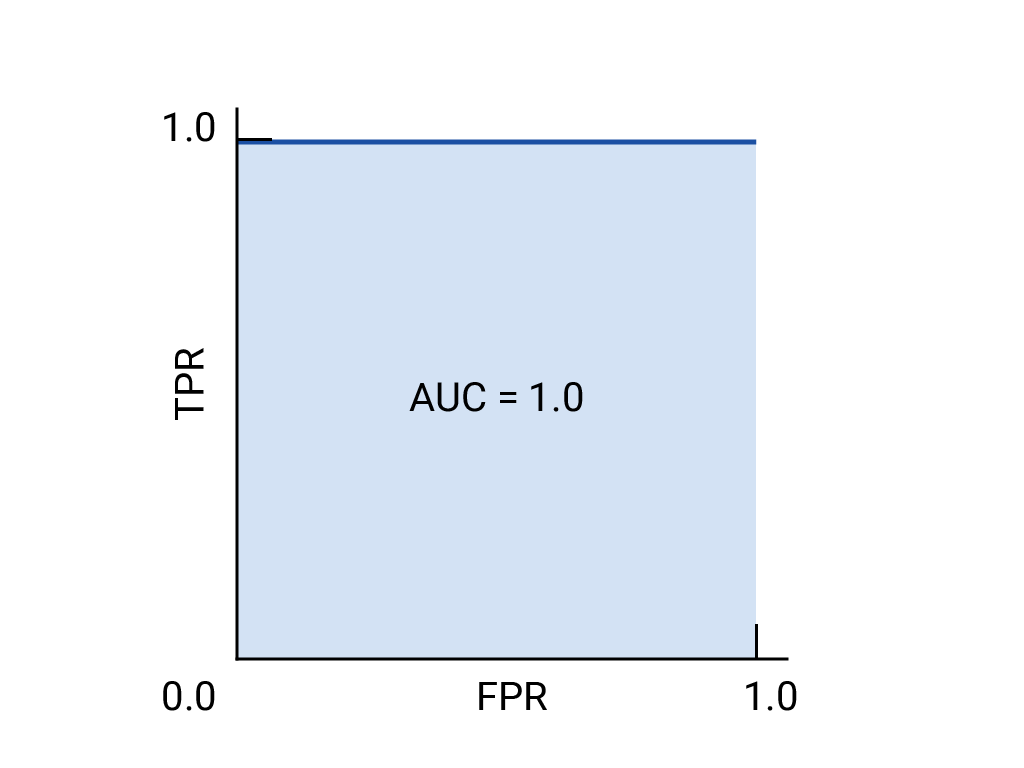
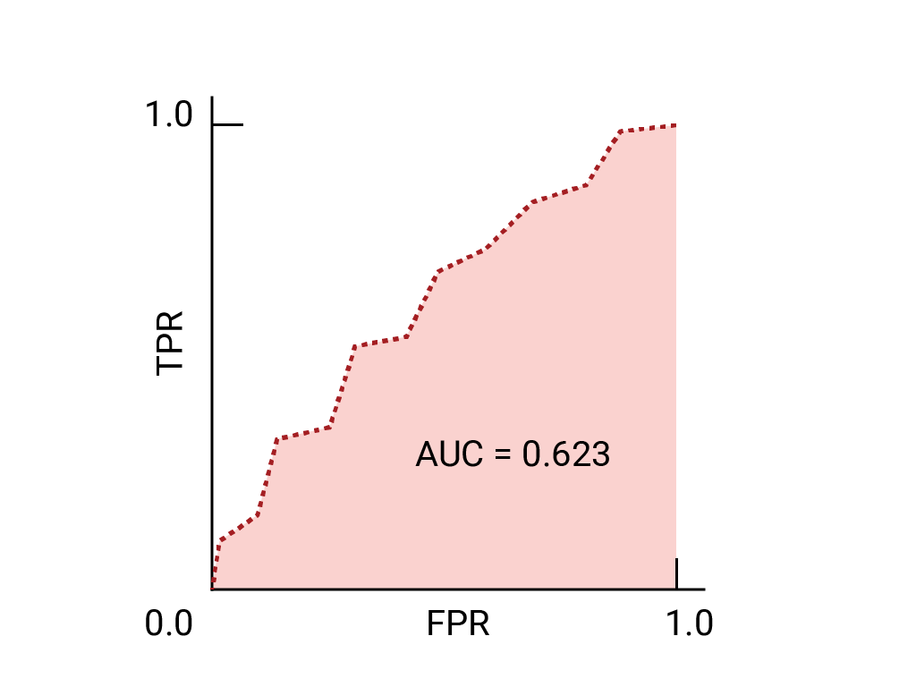
ROC 곡선은 가능한 모든 임곗값 (실제로는 선택한 간격)에서 참양성률 (TPR)과 거짓양성률 (FPR)을 계산한 다음 FPR에 대해 TPR을 그래프로 표시하여 그립니다. 특정 임계값에서 TPR이 1.0이고 FPR이 0.0인 완벽한 모델은 다른 모든 임계값을 무시하는 경우 (0, 1) 지점으로 나타낼 수 있으며, 다음과 같이 나타낼 수도 있습니다.
그림 1. 가상의 완벽한 모델의 ROC 및 AUC
곡선 아래 영역 (AUC)
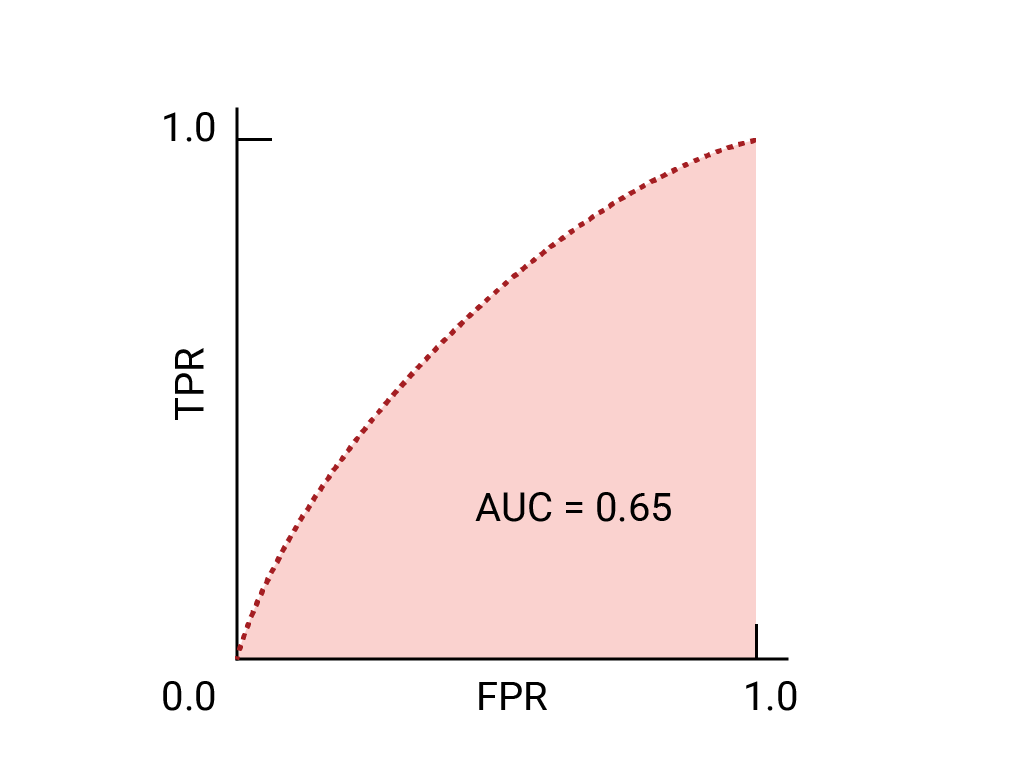
ROC 곡선 아래 영역 (AUC)은 무작위로 선택한 양성 예시와 음성 예시가 주어지면 모델이 양성 예시를 음성 예시보다 높은 순위로 매길 확률을 나타냅니다.
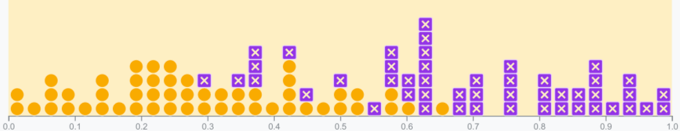
위의 완벽한 모델은 한 변의 길이가 1인 정사각형을 포함하며 곡선 아래 영역 (AUC)이 1.0입니다. 즉, 모델이 무작위로 선택한 양성 예시를 무작위로 선택한 음성 예시보다 정확하게 높은 순위에 올릴 확률은 100% 입니다. 즉, 아래 데이터 포인트의 확산을 보면 AUC는 임계값이 설정된 위치와 관계없이 모델이 무작위로 선택된 정사각형을 무작위로 선택된 원의 오른쪽에 배치할 확률을 나타냅니다.
보다 구체적으로 말하자면 AUC가 1.0인 스팸 분류기는 무작위 스팸 이메일에 무작위로 선택된 정상 이메일보다 스팸일 가능성이 더 높다고 항상 할당합니다. 각 이메일의 실제 분류는 선택한 기준점에 따라 다릅니다.
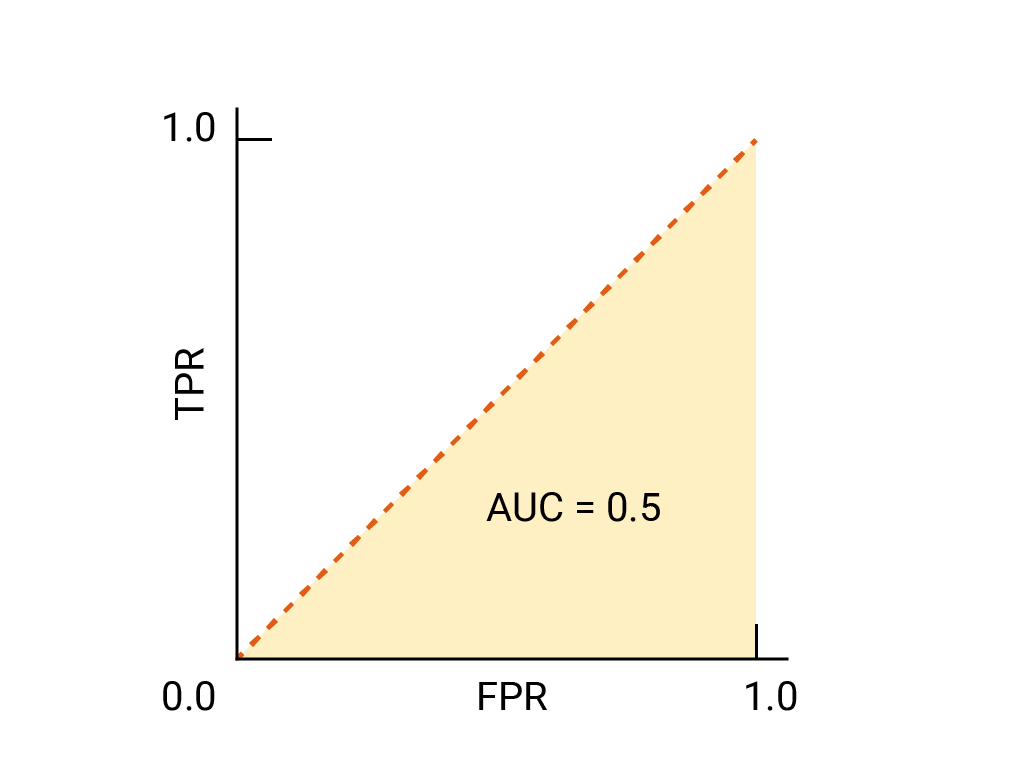
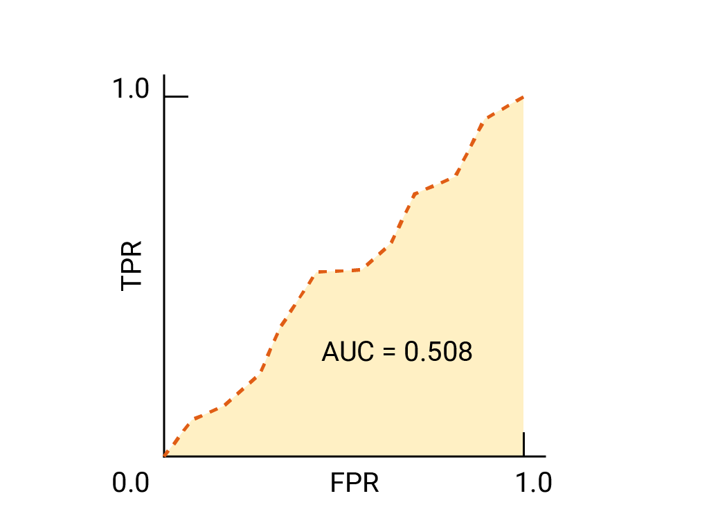
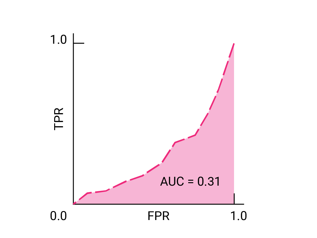
이진 분류기의 경우 무작위 추측이나 동전 던지기와 정확히 동일한 성능을 보이는 모델의 ROC는 (0,0)에서 (1,1)까지의 대각선입니다. AUC는 0.5로, 무작위 양성 예시와 음성 예시를 올바르게 순위 지정할 확률이 50% 임을 나타냅니다.
스팸 분류기 예에서 AUC가 0.5인 스팸 분류기는 무작위 스팸 이메일에 무작위로 선택된 정상 이메일보다 스팸일 확률이 높다는 라벨을 절반의 확률로 할당합니다.
그림 2. 완전히 무작위로 추측한 ROC 및 AUC
(선택사항, 고급) 정밀도-재현율 곡선
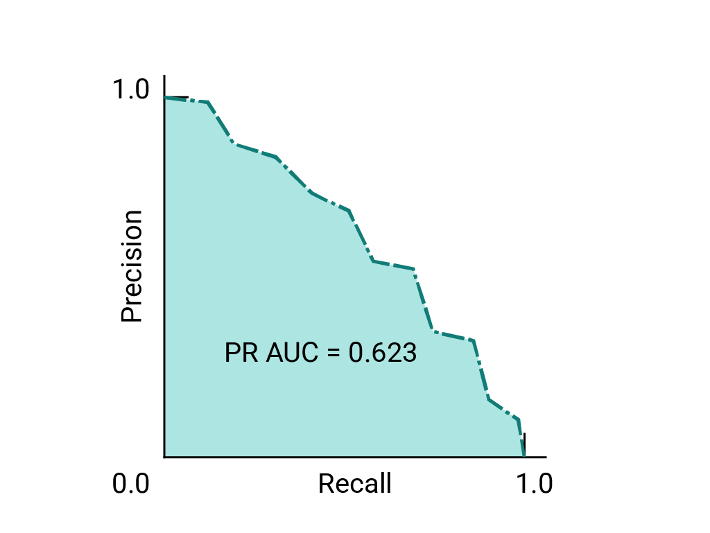
AUC와 ROC는 데이터 세트의 클래스 간에 대략적인 균형이 유지될 때 모델을 비교하는 데 적합합니다. 데이터 세트가 불균형한 경우 정밀도-재현율 곡선 (PRC)과 이러한 곡선 아래의 영역이 모델 성능을 더 잘 비교하여 시각화할 수 있습니다. 정밀도-재현율 곡선은 모든 임곗값에서 정밀도를 y축에, 재현율을 x축에 표시하여 만듭니다.
모델 및 임곗값 선택을 위한 AUC 및 ROC
AUC는 데이터 세트의 균형이 대략 맞는 한 두 가지 모델의 성능을 비교하는 데 유용한 측정항목입니다. 일반적으로 곡선 아래의 면적이 더 큰 모델이 더 좋습니다.
그림 3. 두 가상 모델의 ROC 및 AUC AUC가 더 큰 오른쪽의 곡선이 두 모델 중 더 우수한 모델을 나타냅니다.
ROC 곡선에서 (0,1)에 가장 가까운 점은 특정 모델에 가장 적합한 임곗값의 범위를 나타냅니다. 기준점, 혼동 행렬, 측정항목 선택 및 절충사항 섹션에서 설명한 대로 선택하는 기준점은 특정 사용 사례에 가장 중요한 측정항목에 따라 다릅니다. 다음 다이어그램의 A, B, C 지점은 각각 임곗값을 나타냅니다.
그림 4. 임곗값을 나타내는 라벨이 지정된 점 3개
거짓양성 (거짓 경보)의 비용이 매우 큰 경우 TPR이 감소하더라도 A 지점의 임계값과 같이 FPR이 더 낮은 임계값을 선택하는 것이 좋습니다. 반대로 거짓양성은 비용이 적게 들고 거짓음성(누락된 참양성)은 비용이 많이 드는 경우 TPR을 극대화하는 점 C의 기준점이 더 나을 수 있습니다. 비용이 거의 비슷하다면 B 지점이 TPR과 FPR 간의 균형을 가장 잘 유지할 수 있습니다.
이전에 본 데이터의 ROC 곡선은 다음과 같습니다.
연습: 학습 내용 점검하기
실제로 ROC 곡선은 위의 그림보다 훨씬 불규칙합니다. ROC 곡선과 AUC로 표시된 다음 모델 중 성능이 가장 좋은 모델은 무엇인가요?
이 모델의 AUC가 가장 높으며 이는 가장 우수한 성능과 일치합니다.
다음 중 무작위보다 성능이 나쁜 모델은 무엇인가요?
이 모델의 AUC는 0.5 미만이므로 우연보다 성능이 떨어집니다.
이 모델은 무작위보다 약간 우수한 실적을 보입니다.
이 모델은 확률과 동일하게 작동합니다.
이는 가상의 완벽한 분류기입니다.
(선택사항, 고급) 보너스 문제
이전 질문의 무작위보다 실적이 나쁜 모델을 무작위보다 실적이 우수하도록 만들기 위해 다음 중 어떤 변경사항을 적용할 수 있나요?
예측을 반전하여 1 예측이 0이 되고 0 예측이 1이 되도록 합니다.
바이너리 분류기가 예시를 우연보다 더 자주 잘못된 클래스에 배치하는 경우 클래스 라벨을 전환하면 모델을 다시 학습하지 않아도 즉시 예측 정확도가 우연보다 높아집니다.
항상 음성 클래스를 예측하도록 합니다.
이렇게 하면 실적이 우연히 개선될 수도 있고 그렇지 않을 수도 있습니다. 또한 정확성 섹션에서 설명한 대로 유용한 모델이 아닙니다.
항상 포지티브 클래스를 예측하도록 합니다.
이렇게 하면 실적이 우연히 개선될 수도 있고 그렇지 않을 수도 있습니다. 또한 정확성 섹션에서 설명한 대로 유용한 모델이 아닙니다.
비즈니스상 중요한 이메일을 스팸 폴더로 보내는 것보다 일부 스팸이 받은편지함으로 도착하도록 허용하는 것이 더 나은 상황을 예로 들 수 있습니다. 포지티브 클래스가 스팸이고 네거티브 클래스가 스팸이 아닌 이 상황에 맞게 스팸 분류기를 학습했습니다.
분류기의 ROC 곡선에서 다음 중 어느 지점이 더 바람직한가요?
지점 A
이 사용 사례에서는 참양성도 감소하더라도 거짓양성을 최소화하는 것이 좋습니다.
지점 B
이 임곗값은 참양성과 거짓양성의 균형을 유지합니다.
점 C
이 임계값은 거짓양성 (스팸으로 신고된 더 많은 정상 이메일)을 늘리는 대신 참양성 (더 많은 스팸 신고)을 극대화합니다.
[null,null,["최종 업데이트: 2025-05-23(UTC)"],[],[],null,["# Classification: ROC and AUC\n\nThe previous section presented a set of model metrics, all calculated at a\nsingle classification threshold value. But if you want to evaluate a\nmodel's quality across all possible thresholds, you need different tools.\n\nReceiver-operating characteristic curve (ROC)\n---------------------------------------------\n\nThe [**ROC curve**](/machine-learning/glossary#roc-receiver-operating-characteristic-curve)\nis a visual representation of model performance across all thresholds.\nThe long version of the name, receiver operating characteristic, is a holdover\nfrom WWII radar detection.\n\nThe ROC curve is drawn by calculating the true positive rate (TPR)\nand false positive rate (FPR) at every possible threshold (in practice, at\nselected intervals), then graphing TPR over FPR. A perfect model,\nwhich at some threshold has a TPR of 1.0 and a FPR of 0.0, can\nbe represented by either a point at\n(0, 1) if all other thresholds are ignored, or by the following:\n**Figure 1.** ROC and AUC of a hypothetical perfect model.\n\nArea under the curve (AUC)\n--------------------------\n\nThe [**area under the ROC curve (AUC)**](/machine-learning/glossary#AUC)\nrepresents the probability that the model,\nif given a randomly chosen positive and negative example, will rank the\npositive higher than the negative.\n\nThe perfect model above, containing a square with sides of length 1, has an\narea under the curve (AUC) of 1.0. This means there is a 100% probability that\nthe model will correctly rank a randomly chosen positive example higher than a\nrandomly chosen negative example. In other words, looking at the spread of\ndata points below, AUC gives the probability that the model will place a\nrandomly chosen square to the right of a randomly chosen circle, independent of\nwhere the threshold is set.\n**Figure 2.** A spread of predictions for a binary classification model. AUC is the chance a randomly chosen square is positioned to the right of a randomly chosen circle.\n\nIn more concrete terms, a spam classifier with AUC\nof 1.0 always assigns a random spam email a higher probability of being\nspam than a random legitimate email. The actual classification of each\nemail depends on the threshold that you choose.\n\nFor a binary classifier, a model that does exactly as well as random guesses or\ncoin flips has a ROC that is a diagonal line from (0,0) to (1,1). The AUC is\n0.5, representing a 50% probability of correctly ranking a random positive and\nnegative example.\n\nIn the spam classifier example, a spam classifier with AUC of 0.5 assigns\na random spam email a higher probability of being spam than a random\nlegitimate email only half the time.\n**Figure 3.** ROC and AUC of completely random guesses. \n\n#### (Optional, advanced) Precision-recall curve\n\nAUC and ROC work well for comparing models when the dataset is roughly\nbalanced between classes. When the dataset is imbalanced, precision-recall\ncurves (PRCs) and the area under those curves may offer a better comparative\nvisualization of model performance. Precision-recall curves are created by\nplotting precision on the y-axis and recall on the x-axis across all\nthresholds.\n\nAUC and ROC for choosing model and threshold\n--------------------------------------------\n\nAUC is a useful measure for comparing the performance of two different models,\nas long as the dataset is roughly balanced. The model with greater area under\nthe curve is generally the better one.\n**Figure 4.** ROC and AUC of two hypothetical models. The curve on the right, with a greater AUC, represents the better of the two models.\n\nThe points on a ROC curve closest to (0,1) represent a range of the\nbest-performing thresholds for the given model. As discussed in the\n[Thresholds](/machine-learning/crash-course/classification/thresholding),\n[Confusion matrix](/machine-learning/crash-course/classification/thresholding#confusion_matrix)\nand\n[Choice of metric and tradeoffs](/machine-learning/crash-course/classification/accuracy-precision-recall#choice_of_metric_and_tradeoffs)\nsections, the threshold you choose depends on which metric is most important to\nthe specific use case. Consider the points A, B, and C in the following\ndiagram, each representing a threshold:\n**Figure 5.** Three labeled points representing thresholds.\n\nIf false positives (false alarms) are highly costly, it may make sense to\nchoose a threshold that gives a lower FPR, like the one at point A, even if TPR\nis reduced. Conversely, if false positives are cheap and false negatives\n(missed true positives) highly costly, the threshold for point C, which\nmaximizes TPR, may be preferable. If the costs are roughly equivalent, point B\nmay offer the best balance between TPR and FPR.\n\nHere is the ROC curve for the data we have seen before:\n\nExercise: Check your understanding\n----------------------------------\n\nIn practice, ROC curves are much less regular than the illustrations given above. Which of the following models, represented by their ROC curve and AUC, has the best performance? \nThis model has the highest AUC, which corresponds with the best performance. \nWhich of the following models performs worse than chance? \nThis model has an AUC lower than 0.5, which means it performs worse than chance. \nThis model performs slightly better than chance. \nThis model performs the same as chance. \nThis is a hypothetical perfect classifier. \n\n#### (Optional, advanced) Bonus question\n\nWhich of the following changes can be made to the worse-than-chance model in the previous question to cause it to perform better than chance? \nReverse the predictions, so predictions of **1** become **0** , and predictions of **0** become **1**. \nIf a binary classifier reliably puts examples in the wrong classes more often than chance, switching the class label immediately makes its predictions better than chance without having to retrain the model. \nHave it always predict the negative class. \nThis may or may not improve performance above chance. Also, as discussed in the [Accuracy](/machine-learning/crash-course/classification/accuracy-precision-recall#accuracy) section, this isn't a useful model. \nHave it always predict the positive class. \nThis may or may not improve performance above chance. Also, as discussed in the [Accuracy](/machine-learning/crash-course/classification/accuracy-precision-recall#accuracy) section, this isn't a useful model.\n\n\u003cbr /\u003e\n\nImagine a situation where it's better to allow some spam to reach the\ninbox than to send a business-critical email to the spam folder. You've\ntrained a spam classifier for this situation where the positive class is\nspam and the negative class is not-spam.\nWhich of the following points\non the ROC curve for your classifier is preferable? \nPoint A \nIn this use case, it's better to minimize false positives, even if true positives also decrease. \nPoint B \nThis threshold balances true and false positives. \nPoint C \nThis threshold maximizes true positives (flags more spam) at a cost of more false positives (more legitimate emails flagged as spam).\n| **Key terms:**\n|\n| - [Area under the ROC curve (AUC)](/machine-learning/glossary#AUC)\n- [ROC curve](/machine-learning/glossary#roc-receiver-operating-characteristic-curve) \n[Help Center](https://support.google.com/machinelearningeducation)"]]