با مجموعهها، منظم بمانید
ذخیره و طبقهبندی محتوا براساس اولویتهای شما.
بخش قبلی مجموعهای از معیارهای مدل را ارائه میکند که همگی در یک مقدار آستانه طبقهبندی محاسبه شدهاند. اما اگر می خواهید کیفیت یک مدل را در تمام آستانه های ممکن ارزیابی کنید، به ابزارهای مختلفی نیاز دارید.
منحنی مشخصه عملکرد گیرنده (ROC)
منحنی ROC یک نمایش بصری از عملکرد مدل در تمام آستانه ها است. نسخه طولانی این نام، مشخصه عملکرد گیرنده، از کشف راداری جنگ جهانی دوم باقی مانده است.
منحنی ROC با محاسبه نرخ مثبت واقعی (TPR) و نرخ مثبت کاذب (FPR) در هر آستانه ممکن (در عمل، در فواصل زمانی انتخاب شده)، سپس نمودار TPR بر روی FPR ترسیم می شود. یک مدل کامل، که در برخی از آستانه ها دارای TPR 1.0 و FPR 0.0 است، می تواند با یک نقطه در (0، 1) در صورتی که همه آستانه های دیگر نادیده گرفته شوند، یا با موارد زیر نشان داده شود:
شکل 1. ROC و AUC یک مدل کامل فرضی.
مساحت زیر منحنی (AUC)
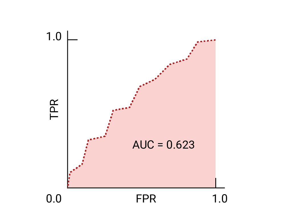
سطح زیر منحنی ROC (AUC) نشان دهنده این احتمال است که مدل، اگر به طور تصادفی یک مثال مثبت و منفی انتخاب شود، مثبت را بالاتر از منفی قرار دهد.
مدل کامل بالا، شامل مربعی با اضلاع به طول 1، دارای مساحت زیر منحنی (AUC) 1.0 است. این به این معنی است که احتمال 100٪ وجود دارد که مدل به درستی یک مثال مثبت انتخاب شده به طور تصادفی را بالاتر از یک مثال منفی تصادفی انتخاب کند. به عبارت دیگر، با نگاهی به گسترش نقاط داده در زیر، AUC این احتمال را می دهد که مدل یک مربع به طور تصادفی انتخاب شده را در سمت راست دایره ای که به طور تصادفی انتخاب شده است، مستقل از جایی که آستانه تنظیم شده است، قرار دهد.
به عبارت دقیق تر، یک طبقه بندی کننده هرزنامه با AUC 1.0 همیشه به یک ایمیل هرزنامه تصادفی احتمال بیشتری نسبت به ایمیل های قانونی تصادفی برای اسپم بودن اختصاص می دهد. طبقه بندی واقعی هر ایمیل به آستانه ای که انتخاب می کنید بستگی دارد.
برای یک طبقهبندیکننده باینری، مدلی که دقیقاً به خوبی حدسهای تصادفی یا چرخش سکه انجام میدهد، دارای یک ROC است که یک خط مورب از (۰،۰) تا (۱،۱) است. AUC 0.5 است که نشان دهنده 50% احتمال رتبه بندی صحیح یک مثال تصادفی مثبت و منفی است.
در مثال طبقهبندی کننده هرزنامه، یک طبقهبندی کننده هرزنامه با AUC 0.5 به یک ایمیل هرزنامه تصادفی احتمال بیشتری برای اسپم بودن نسبت به ایمیلهای قانونی تصادفی اختصاص میدهد.
شکل 2. ROC و AUC از حدس های کاملا تصادفی.
(اختیاری، پیشرفته) منحنی فراخوان دقیق
AUC و ROC برای مقایسه مدلها زمانی که مجموعه داده تقریباً بین کلاسها متعادل است، به خوبی کار میکنند. هنگامی که مجموعه داده نامتعادل است، منحنی های فراخوان دقیق (PRC) و ناحیه زیر آن منحنی ها ممکن است تجسم مقایسه ای بهتری از عملکرد مدل ارائه دهند. منحنیهای فراخوان دقیق با ترسیم دقت بر روی محور y و فراخوانی در محور x در تمام آستانهها ایجاد میشوند.
AUC و ROC برای انتخاب مدل و آستانه
AUC یک معیار مفید برای مقایسه عملکرد دو مدل مختلف است، تا زمانی که مجموعه داده تقریباً متعادل باشد. مدلی که سطح زیر منحنی بیشتری دارد معمولاً مدل بهتری است.
شکل 3. ROC و AUC دو مدل فرضی. منحنی سمت راست، با AUC بیشتر، نشاندهنده بهتری از دو مدل است.
نقاط روی یک منحنی ROC نزدیکترین به (0،1) طیفی از آستانههای با بهترین عملکرد را برای مدل داده شده نشان میدهند. همانطور که در بخش آستانه ها ، ماتریس سردرگمی و انتخاب متریک و مبادلات بحث شد، آستانه ای که انتخاب می کنید بستگی به این دارد که کدام متریک برای مورد استفاده خاص مهم است. نقاط A، B و C را در نمودار زیر در نظر بگیرید که هر کدام یک آستانه را نشان می دهند:
شکل 4. سه نقطه برچسب گذاری شده که آستانه ها را نشان می دهد.
اگر موارد مثبت کاذب (آژیرهای کاذب) بسیار پرهزینه هستند، ممکن است منطقی باشد که آستانه ای را انتخاب کنید که FPR کمتری می دهد، مانند آنچه در نقطه A است، حتی اگر TPR کاهش یابد. برعکس، اگر مثبت های کاذب ارزان و منفی های کاذب (مثبت های واقعی از دست رفته) بسیار پرهزینه باشند، آستانه نقطه C، که TPR را به حداکثر می رساند، ممکن است ارجح باشد. اگر هزینه ها تقریباً معادل باشند، نقطه B ممکن است بهترین تعادل را بین TPR و FPR ارائه دهد.
در اینجا منحنی ROC برای دادههایی که قبلا دیدهایم است:
تمرین: درک خود را بررسی کنید
در عمل، منحنی های ROC بسیار کمتر از تصاویر ارائه شده در بالا منظم هستند. کدام یک از مدل های زیر که با منحنی ROC و AUC نشان داده می شوند، بهترین عملکرد را دارند؟
این مدل دارای بالاترین AUC است که با بهترین عملکرد مطابقت دارد.
کدام یک از مدل های زیر بدتر از شانس عمل می کند؟
این مدل دارای AUC کمتر از 0.5 است که به معنای عملکرد بدتر از شانس است.
این مدل کمی بهتر از شانس عمل می کند.
این مدل مانند شانس عمل می کند.
این یک طبقه بندی کننده کامل فرضی است.
(اختیاری، پیشرفته) سوال جایزه
کدام یک از تغییرات زیر را می توان در مدل بدتر از شانس در سوال قبل ایجاد کرد تا عملکرد آن بهتر از شانس باشد؟
پیش بینی ها را معکوس کنید، بنابراین پیش بینی های 1 تبدیل به 0 و پیش بینی های 0 تبدیل به 1 می شوند.
اگر یک طبقهبندیکننده باینری بهطور قابل اعتمادی نمونهها را بیشتر از شانس در کلاسهای اشتباه قرار میدهد، تغییر برچسب کلاس بلافاصله بدون نیاز به آموزش مجدد مدل، پیشبینیهای آن را بهتر از شانس میکند.
آیا همیشه کلاس منفی را پیش بینی کند.
این ممکن است عملکرد بالاتر از شانس را بهبود بخشد یا خیر. همچنین، همانطور که در بخش دقت بحث شد، این مدل مفیدی نیست.
آیا آن را همیشه پیش بینی طبقه مثبت است.
این ممکن است عملکرد بالاتر از شانس را بهبود بخشد یا خیر. همچنین، همانطور که در بخش دقت بحث شد، این مدل مفیدی نیست.
وضعیتی را تصور کنید که در آن بهتر است اجازه دهید مقداری هرزنامه به صندوق ورودی برسد تا اینکه یک ایمیل مهم تجاری به پوشه هرزنامه ارسال کنید. شما یک طبقهبندی کننده هرزنامه را برای این وضعیت آموزش دادهاید که در آن کلاس مثبت هرزنامه است و کلاس منفی هرزنامه نیست. کدام یک از نقاط زیر در منحنی ROC برای طبقه بندی کننده شما ارجح است؟
نقطه الف
در این مورد، بهتر است که مثبت های کاذب را به حداقل برسانید، حتی اگر مثبت های واقعی نیز کاهش پیدا کنند.
نقطه B
این آستانه بین مثبتهای درست و نادرست تعادل برقرار میکند.
نقطه ج
این آستانه، موارد مثبت واقعی (پرچمگذاری هرزنامههای بیشتر) را با هزینه بیشتر مثبت کاذب (ایمیلهای قانونی بیشتر که به عنوان هرزنامه پرچمگذاری شدهاند) به حداکثر میرساند.
تاریخ آخرین بهروزرسانی 2025-05-23 بهوقت ساعت هماهنگ جهانی.
[null,null,["تاریخ آخرین بهروزرسانی 2025-05-23 بهوقت ساعت هماهنگ جهانی."],[],[],null,["# Classification: ROC and AUC\n\nThe previous section presented a set of model metrics, all calculated at a\nsingle classification threshold value. But if you want to evaluate a\nmodel's quality across all possible thresholds, you need different tools.\n\nReceiver-operating characteristic curve (ROC)\n---------------------------------------------\n\nThe [**ROC curve**](/machine-learning/glossary#roc-receiver-operating-characteristic-curve)\nis a visual representation of model performance across all thresholds.\nThe long version of the name, receiver operating characteristic, is a holdover\nfrom WWII radar detection.\n\nThe ROC curve is drawn by calculating the true positive rate (TPR)\nand false positive rate (FPR) at every possible threshold (in practice, at\nselected intervals), then graphing TPR over FPR. A perfect model,\nwhich at some threshold has a TPR of 1.0 and a FPR of 0.0, can\nbe represented by either a point at\n(0, 1) if all other thresholds are ignored, or by the following:\n**Figure 1.** ROC and AUC of a hypothetical perfect model.\n\nArea under the curve (AUC)\n--------------------------\n\nThe [**area under the ROC curve (AUC)**](/machine-learning/glossary#AUC)\nrepresents the probability that the model,\nif given a randomly chosen positive and negative example, will rank the\npositive higher than the negative.\n\nThe perfect model above, containing a square with sides of length 1, has an\narea under the curve (AUC) of 1.0. This means there is a 100% probability that\nthe model will correctly rank a randomly chosen positive example higher than a\nrandomly chosen negative example. In other words, looking at the spread of\ndata points below, AUC gives the probability that the model will place a\nrandomly chosen square to the right of a randomly chosen circle, independent of\nwhere the threshold is set.\n**Figure 2.** A spread of predictions for a binary classification model. AUC is the chance a randomly chosen square is positioned to the right of a randomly chosen circle.\n\nIn more concrete terms, a spam classifier with AUC\nof 1.0 always assigns a random spam email a higher probability of being\nspam than a random legitimate email. The actual classification of each\nemail depends on the threshold that you choose.\n\nFor a binary classifier, a model that does exactly as well as random guesses or\ncoin flips has a ROC that is a diagonal line from (0,0) to (1,1). The AUC is\n0.5, representing a 50% probability of correctly ranking a random positive and\nnegative example.\n\nIn the spam classifier example, a spam classifier with AUC of 0.5 assigns\na random spam email a higher probability of being spam than a random\nlegitimate email only half the time.\n**Figure 3.** ROC and AUC of completely random guesses. \n\n#### (Optional, advanced) Precision-recall curve\n\nAUC and ROC work well for comparing models when the dataset is roughly\nbalanced between classes. When the dataset is imbalanced, precision-recall\ncurves (PRCs) and the area under those curves may offer a better comparative\nvisualization of model performance. Precision-recall curves are created by\nplotting precision on the y-axis and recall on the x-axis across all\nthresholds.\n\nAUC and ROC for choosing model and threshold\n--------------------------------------------\n\nAUC is a useful measure for comparing the performance of two different models,\nas long as the dataset is roughly balanced. The model with greater area under\nthe curve is generally the better one.\n**Figure 4.** ROC and AUC of two hypothetical models. The curve on the right, with a greater AUC, represents the better of the two models.\n\nThe points on a ROC curve closest to (0,1) represent a range of the\nbest-performing thresholds for the given model. As discussed in the\n[Thresholds](/machine-learning/crash-course/classification/thresholding),\n[Confusion matrix](/machine-learning/crash-course/classification/thresholding#confusion_matrix)\nand\n[Choice of metric and tradeoffs](/machine-learning/crash-course/classification/accuracy-precision-recall#choice_of_metric_and_tradeoffs)\nsections, the threshold you choose depends on which metric is most important to\nthe specific use case. Consider the points A, B, and C in the following\ndiagram, each representing a threshold:\n**Figure 5.** Three labeled points representing thresholds.\n\nIf false positives (false alarms) are highly costly, it may make sense to\nchoose a threshold that gives a lower FPR, like the one at point A, even if TPR\nis reduced. Conversely, if false positives are cheap and false negatives\n(missed true positives) highly costly, the threshold for point C, which\nmaximizes TPR, may be preferable. If the costs are roughly equivalent, point B\nmay offer the best balance between TPR and FPR.\n\nHere is the ROC curve for the data we have seen before:\n\nExercise: Check your understanding\n----------------------------------\n\nIn practice, ROC curves are much less regular than the illustrations given above. Which of the following models, represented by their ROC curve and AUC, has the best performance? \nThis model has the highest AUC, which corresponds with the best performance. \nWhich of the following models performs worse than chance? \nThis model has an AUC lower than 0.5, which means it performs worse than chance. \nThis model performs slightly better than chance. \nThis model performs the same as chance. \nThis is a hypothetical perfect classifier. \n\n#### (Optional, advanced) Bonus question\n\nWhich of the following changes can be made to the worse-than-chance model in the previous question to cause it to perform better than chance? \nReverse the predictions, so predictions of **1** become **0** , and predictions of **0** become **1**. \nIf a binary classifier reliably puts examples in the wrong classes more often than chance, switching the class label immediately makes its predictions better than chance without having to retrain the model. \nHave it always predict the negative class. \nThis may or may not improve performance above chance. Also, as discussed in the [Accuracy](/machine-learning/crash-course/classification/accuracy-precision-recall#accuracy) section, this isn't a useful model. \nHave it always predict the positive class. \nThis may or may not improve performance above chance. Also, as discussed in the [Accuracy](/machine-learning/crash-course/classification/accuracy-precision-recall#accuracy) section, this isn't a useful model.\n\n\u003cbr /\u003e\n\nImagine a situation where it's better to allow some spam to reach the\ninbox than to send a business-critical email to the spam folder. You've\ntrained a spam classifier for this situation where the positive class is\nspam and the negative class is not-spam.\nWhich of the following points\non the ROC curve for your classifier is preferable? \nPoint A \nIn this use case, it's better to minimize false positives, even if true positives also decrease. \nPoint B \nThis threshold balances true and false positives. \nPoint C \nThis threshold maximizes true positives (flags more spam) at a cost of more false positives (more legitimate emails flagged as spam).\n| **Key terms:**\n|\n| - [Area under the ROC curve (AUC)](/machine-learning/glossary#AUC)\n- [ROC curve](/machine-learning/glossary#roc-receiver-operating-characteristic-curve) \n[Help Center](https://support.google.com/machinelearningeducation)"]]