Page Summary
-
Gradient descent is an iterative optimization algorithm used to find the best weights and bias for a linear regression model by minimizing the loss function.
-
The process involves repeatedly calculating the loss, determining the direction to adjust weights and bias to reduce loss, and updating the parameters accordingly.
-
A model is considered to have converged when further iterations do not significantly reduce the loss, indicating it has found the weights and bias that produce the lowest possible loss.
-
Loss curves visually represent the model's progress during training, showing how the loss decreases over iterations and helping to identify convergence.
-
Linear models have convex loss functions, ensuring that gradient descent will always find the global minimum, resulting in the best possible model for the given data.
Gradient descent is a mathematical technique that iteratively finds the weights and bias that produce the model with the lowest loss. Gradient descent finds the best weight and bias by repeating the following process for a number of user-defined iterations.
The model begins training with randomized weights and biases near zero, and then repeats the following steps:
Calculate the loss with the current weight and bias.
Determine the direction to move the weights and bias that reduce loss.
Move the weight and bias values a small amount in the direction that reduces loss.
Return to step one and repeat the process until the model can't reduce the loss any further.
The diagram below outlines the iterative steps gradient descent performs to find the weights and bias that produce the model with the lowest loss.
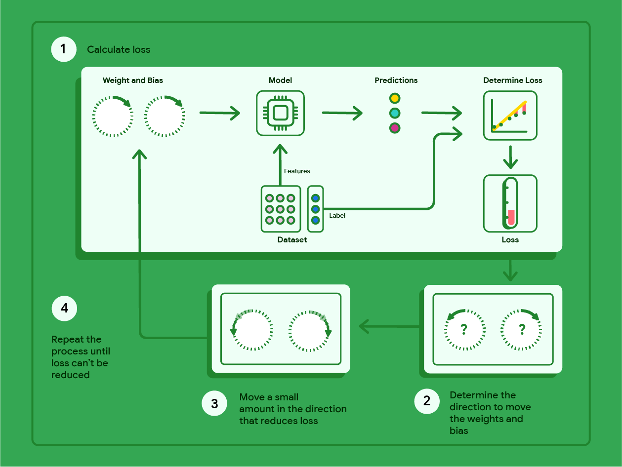
Figure 11. Gradient descent is an iterative process that finds the weights and bias that produce the model with the lowest loss.
Model convergence and loss curves
When training a model, you'll often look at a loss curve to determine if the model has converged. The loss curve shows how the loss changes as the model trains. The following is what a typical loss curve looks like. Loss is on the y-axis and iterations are on the x-axis:
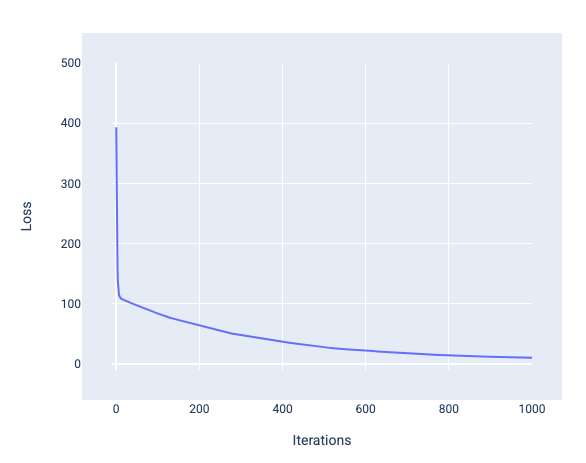
Figure 12. Loss curve showing the model converging around the 1,000th-iteration mark.
You can see that loss dramatically decreases during the first few iterations, then gradually decreases before flattening out around the 1,000th-iteration mark. After 1,000 iterations, we can be mostly certain that the model has converged.
In the following figures, we draw the model at three points during the training process: the beginning, the middle, and the end. Visualizing the model's state at snapshots during the training process solidifies the link between updating the weights and bias, reducing loss, and model convergence.
In the figures, we use the derived weights and bias at a particular iteration to represent the model. In the graph with the data points and the model snapshot, blue loss lines from the model to the data points show the amount of loss. The longer the lines, the more loss there is.
In the following figure, we can see that around the second iteration the model would not be good at making predictions because of the high amount of loss.
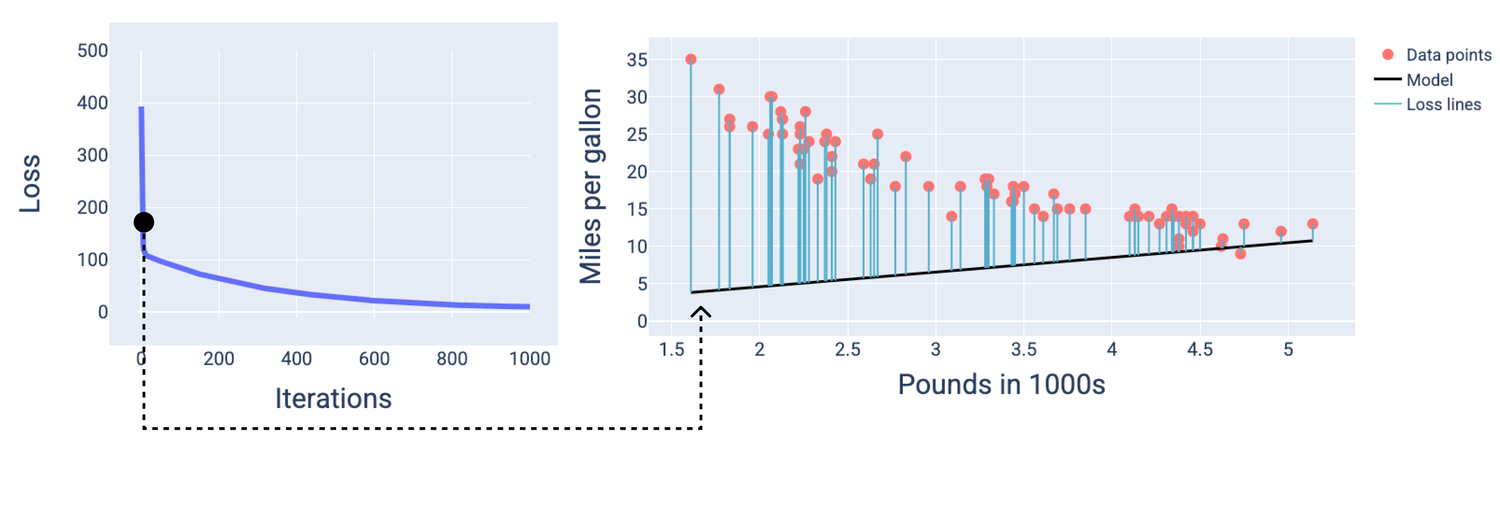
Figure 13. Loss curve and snapshot of the model at the beginning of the training process.
At around the 400th-iteration, we can see that gradient descent has found the weight and bias that produce a better model.
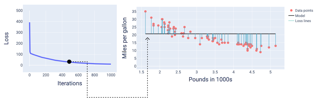
Figure 14. Loss curve and snapshot of model about midway through training.
And at around the 1,000th-iteration, we can see that the model has converged, producing a model with the lowest possible loss.
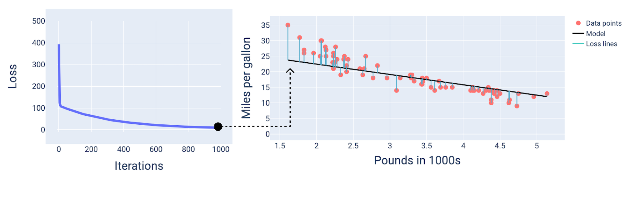
Figure 15. Loss curve and snapshot of the model near the end of the training process.
Exercise: Check your understanding
Convergence and convex functions
The loss functions for linear models always produce a convex surface. As a result of this property, when a linear regression model converges, we know the model has found the weights and bias that produce the lowest loss.
If we graph the loss surface for a model with one feature, we can see its convex shape. The following is the loss surface for a hypothetical miles per gallon dataset. Weight is on the x-axis, bias is on the y-axis, and loss is on the z-axis:
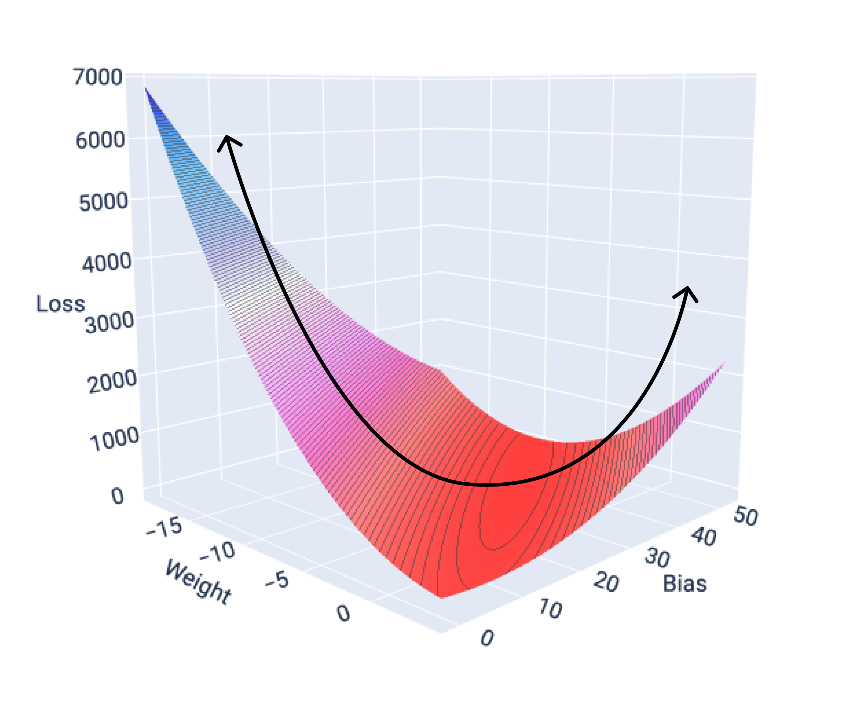
Figure 16. Loss surface that shows its convex shape.
In this example, a weight of -5.44 and bias of 35.94 produce the lowest loss at 5.54:
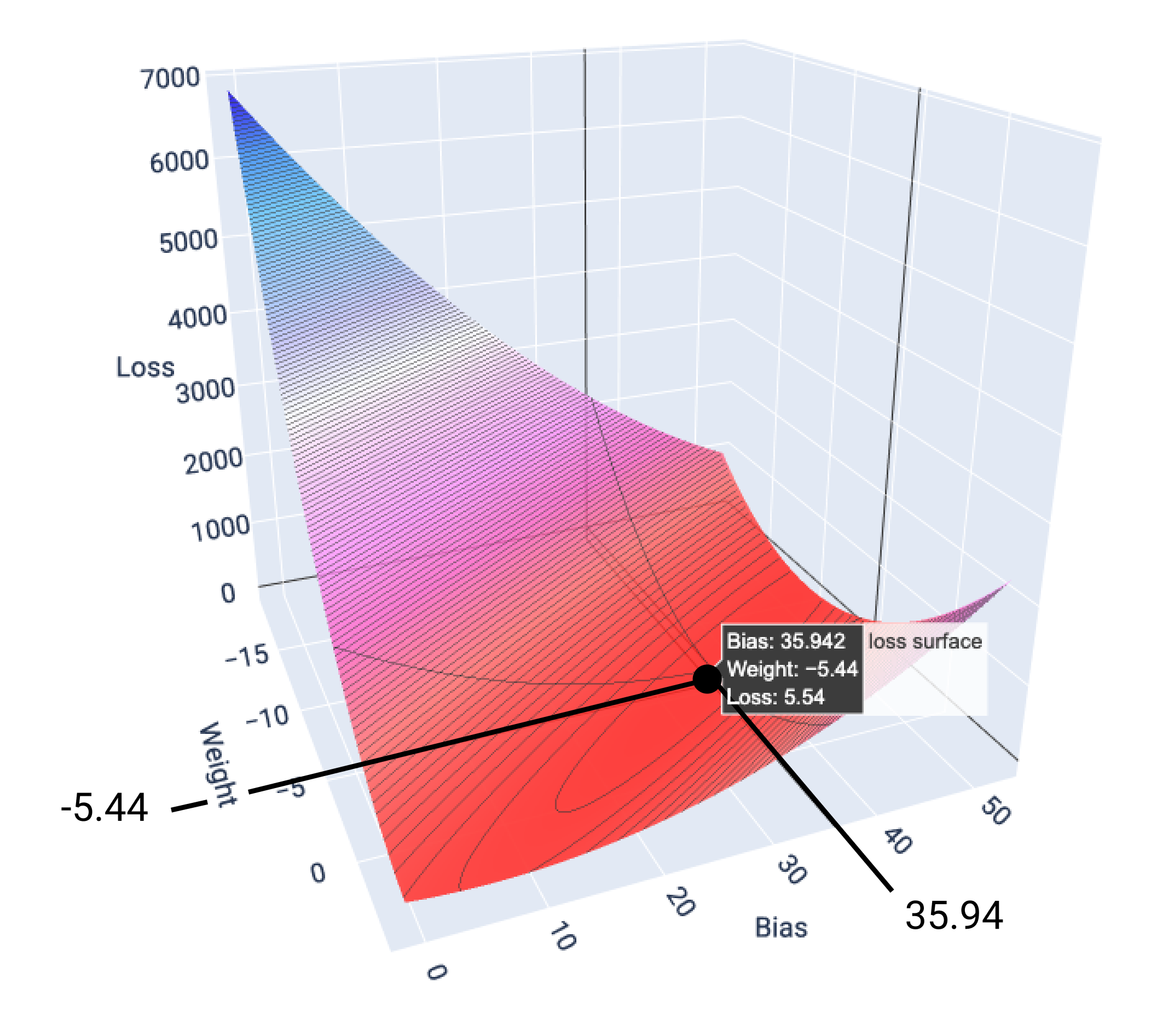
Figure 17. Loss surface showing the weight and bias values that produce the lowest loss.
A linear model converges when it's found the minimum loss. If we graphed the weights and bias points during gradient descent, the points would look like a ball rolling down a hill, finally stopping at the point where there's no more downward slope.
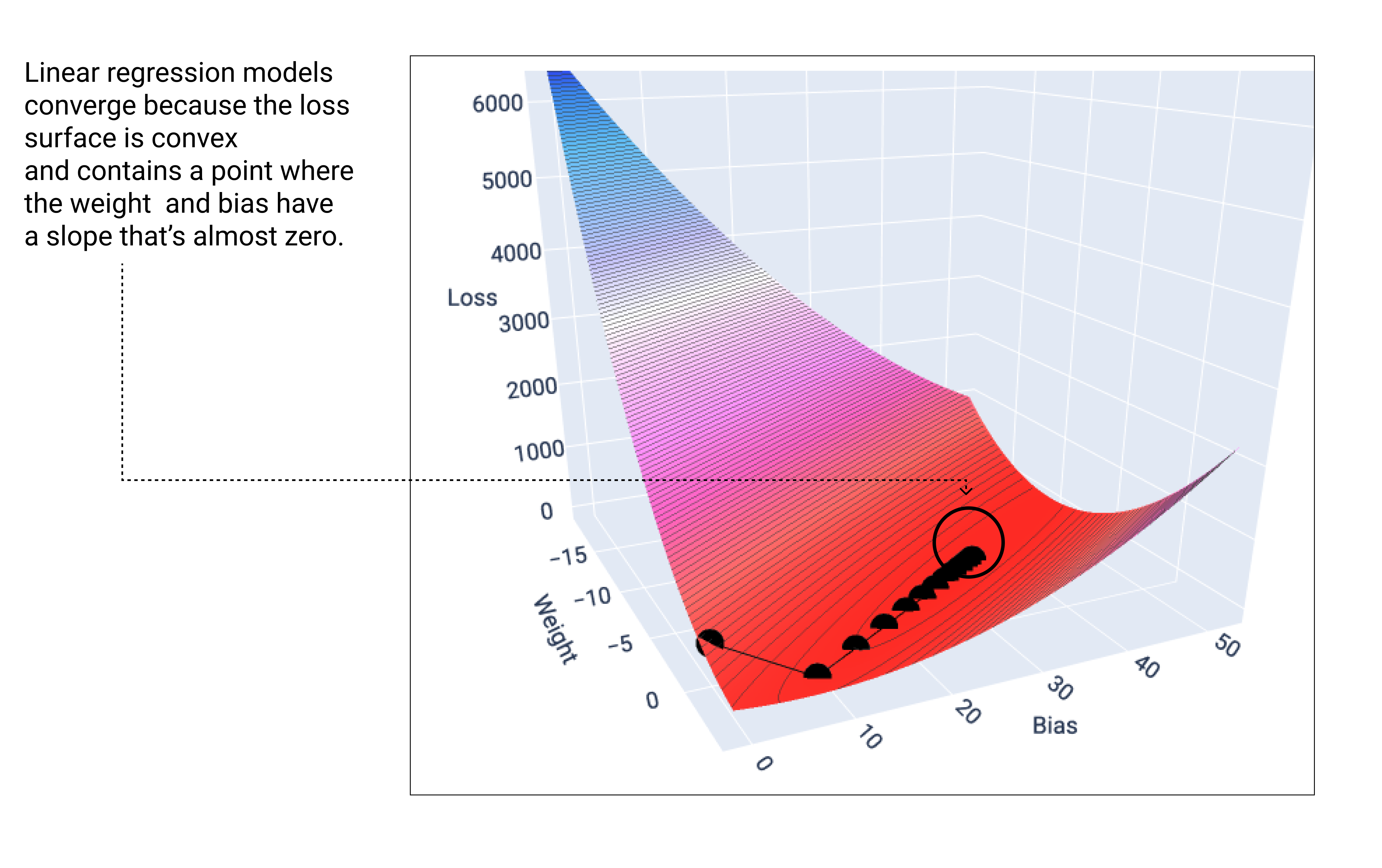
Figure 18. Loss graph showing gradient descent points stopping at the lowest point on the graph.
Notice that the black loss points create the exact shape of the loss curve: a steep decline before gradually sloping down until they've reached the lowest point on the loss surface.
Using the weight and bias values that produce the lowest loss—in this case a weight of -5.44 and a bias of 35.94—we can graph the model to see how well it fits the data:
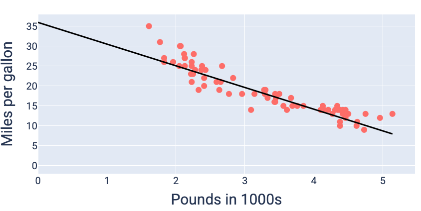
Figure 19. Model graphed using the weight and bias values that produce the lowest loss.
This would be the best model for this dataset because no other weight and bias values produce a model with lower loss.