Numerical data: Polynomial transforms

Sometimes, when the ML practitioner has domain knowledge suggesting that one variable is related to the square, cube, or other power of another variable, it's useful to create a synthetic feature from one of the existing numerical features.

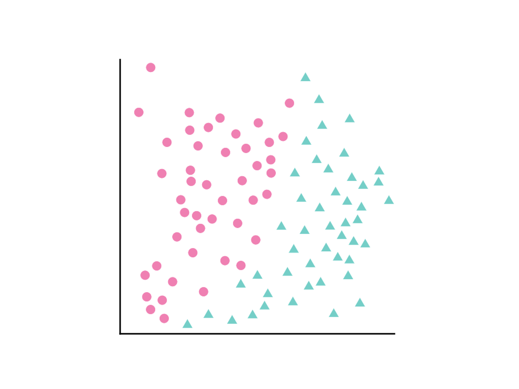
Consider the following spread of data points, where pink circles represent one class or category (for example, a species of tree) and green triangles another class (or species of tree):

Figure 17. Two classes that can't be separated by a line.

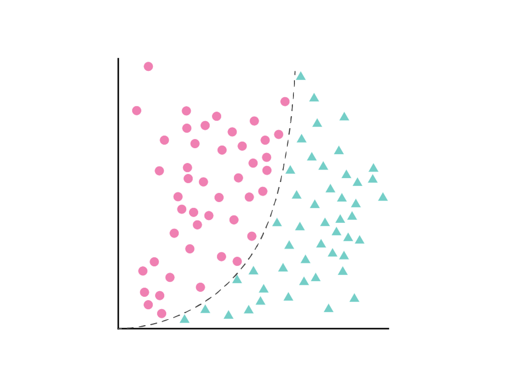
It's not possible to draw a straight line that cleanly separates the two classes, but it is possible to draw a curve that does so:

Figure 18. Separating the classes with y = x².

As discussed in the Linear regression module, a linear model with one feature, $x_1$, is described by the linear equation:

$$y = b + w_1x_1$$

Additional features are handled by the addition of terms \(w_2x_2\), \(w_3x_3\), etc.

Gradient descent finds the weight $w_1$ (or weights \(w_1\), \(w_2\), \(w_3\), in the case of additional features) that minimizes the loss of the model. But the data points shown cannot be separated by a line. What can be done?

It's possible to keep both the linear equation and allow nonlinearity by defining a new term, \(x_2\), that is simply \(x_1\) squared:

$$x_2 = x_1^2$$

This synthetic feature, called a polynomial transform, is treated like any other feature. The previous linear formula becomes:

$$y = b + w_1x_1 + w_2x_2$$

This can still be treated like a linear regression problem, and the weights determined through gradient descent, as usual, despite containing a hidden squared term, the polynomial transform. Without changing how the linear model trains, the addition of a polynomial transform allows the model to separate the data points using a curve of the form $y = b + w_1x + w_2x^2$.

Usually the numerical feature of interest is multiplied by itself, that is, raised to some power. Sometimes an ML practitioner can make an informed guess about the appropriate exponent. For example, many relationships in the physical world are related to squared terms, including acceleration due to gravity, the attenuation of light or sound over distance, and elastic potential energy.

A related concept in categorical data is the feature cross, which more frequently synthesizes two different features.

Key terms:

• Categorical data
• Feature
• Feature cross
• Gradient descent
• Linear regression
• Synthetic feature
• Weight