숫자 데이터: 다항 변환

ML 전문가에게 한 변수가 다른 변수의 제곱, 세제곱 또는 기타 지수와 관련이 있다는 도메인 지식이 있는 경우 기존 숫자 특성 중 하나에서 합성 특성을 만드는 것이 유용합니다.

다음과 같이 데이터 포인트가 퍼져 있는 경우를 생각해 보세요. 분홍색 원은 한 클래스 또는 카테고리 (예: 나무 종)를 나타내고 녹색 삼각형은 다른 클래스 (또는 나무 종)를 나타냅니다.

그림 17. 선으로 구분할 수 없는 두 클래스

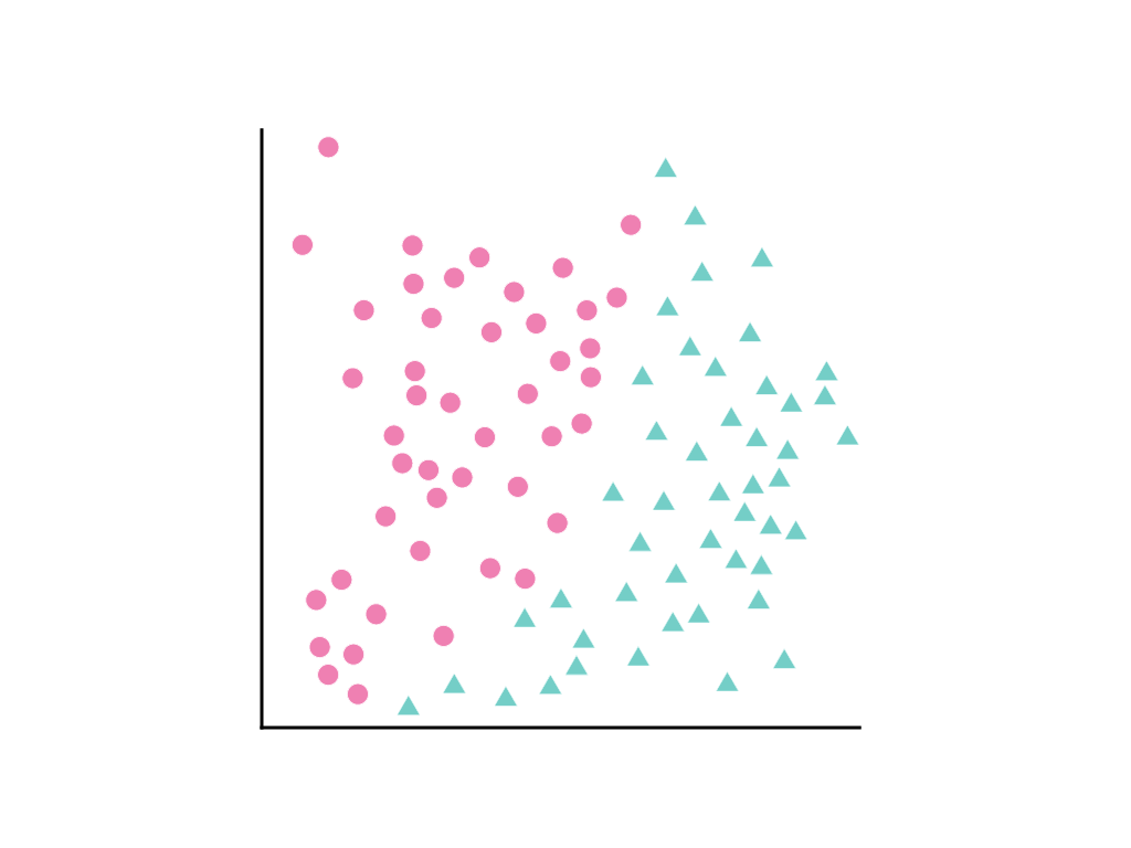
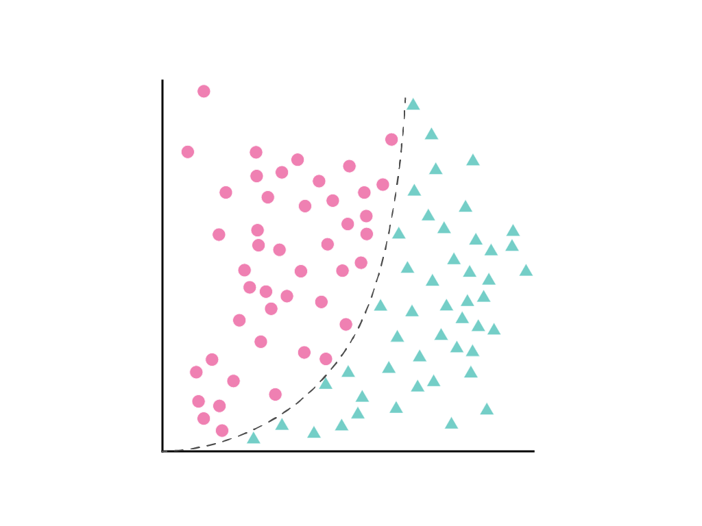
두 클래스를 깔끔하게 구분하는 직선을 그릴 수는 없지만 이를 구분하는 곡선을 그릴 수는 있습니다.

그림 18. y = x²로 클래스를 구분합니다.

선형 회귀 모듈에서 논의한 바와 같이 특성 1개($x_1$)가 있는 선형 모델은 다음과 같은 선형 방정식으로 설명됩니다.

$$y = b + w_1x_1$$

추가 기능은 \(w_2x_2\),\(w_3x_3\)등의 용어를 추가하여 처리됩니다.

경사하강법은 모델의 손실을 최소화하는 가중치 $w_1$ (또는 추가 기능의 경우 가중치\(w_1\), \(w_2\), \(w_3\))를 찾습니다. 하지만 표시된 데이터 포인트는 선으로 구분할 수 없습니다. 어떻게 해야 하나요?

\(x_1\) 제곱된 새로운 용어 \(x_2\)를 정의하여 선형 방정식을 유지하면서 비선형성을 허용할 수 있습니다.

$$x_2 = x_1^2$$

다항식 변환이라고 하는 이 합성 특성은 다른 특성과 마찬가지로 취급됩니다. 이전 선형 수식은 다음과 같이 변경됩니다.

$$y = b + w_1x_1 + w_2x_2$$

여전히 선형 회귀 문제처럼 취급할 수 있으며, 숨겨진 제곱 항인 다항식 변환이 포함되어 있음에도 불구하고 평소와 같이 기울기 하강법을 통해 가중치를 결정할 수 있습니다. 선형 모델의 학습 방식을 변경하지 않고도 다항식 변환을 추가하면 모델이 $y = b + w_1x + w_2x^2$ 형식의 곡선을 사용하여 데이터 포인트를 구분할 수 있습니다.

일반적으로 관심의 대상이 되는 수치적 특징은 자기 자신과 곱해집니다. 즉, 지수로 거듭제곱됩니다. ML 전문가가 적절한 지수에 관해 정보에 입각한 추측을 할 수 있는 경우도 있습니다. 예를 들어 물리적 세계의 많은 관계는 중력으로 인한 가속도, 거리에 따른 빛 또는 소리의 감쇠, 탄성 잠재 에너지를 비롯하여 제곱된 항목과 관련이 있습니다.

지형지물을 변환하여 크기를 변경하는 경우 정규화도 실험해 보세요. 변환 후 정규화하면 모델 성능이 향상될 수 있습니다. 자세한 내용은 숫자 데이터: 정규화를 참고하세요.

범주형 데이터와 관련된 개념은 두 가지 다른 특성을 더 자주 합성하는 특성 교차입니다.

핵심 용어:

• 범주형 데이터
• 기능
• 특성 교차
• 경사하강법
• 선형 회귀
• 합성 지형지물
• 무게