Embeddings: Translating to a lower-dimensional space

An embedding is a relatively low-dimensional space into which you can translate high-dimensional vectors. For a discussion of high-dimensional vs. low-dimensional data, see the Categorical Data module.

Embeddings make it easier to do machine learning on large feature vectors, such as the sparse vectors representing meal items discussed in the previous section. Ideally, an embedding captures some of the semantics of the input by placing inputs that are more similar in meaning closer together in the embedding space. For example, a good embedding would place the word "car" closer to "garage" than to "elephant." An embedding can be trained and reused across models.

To give an idea of how embedding vectors represent information, consider the following one-dimensional representation of the dishes hot dog, pizza, salad, shawarma, and borscht, on a scale of "least like a sandwich" to "most like a sandwich." "Sandwichness" is the single dimension.

Figure 3. Foods along an imagined dimension of "sandwichness."

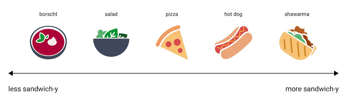
Where on this line would an apple strudel fall? Arguably, it could be placed between hot dog and shawarma. But apple strudel also seems to have an additional dimension of sweetness (how sweet the food is) or dessertness (how much like a dessert the food is) that makes it very different from the other options. The following figure visualizes this by adding a "dessertness" dimension:

Figure 4. Foods plotted by both "sandwichness" and "dessertness."

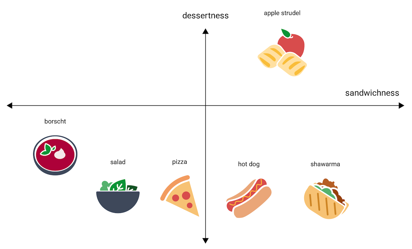
An embedding represents each item in n-dimensional space with n floating-point numbers (typically in the range –1 to 1 or 0 to 1). For example, the embedding in Figure 4 represents each meal item in two-dimensional space with two coordinates. The item "apple strudel" is in the upper-right quadrant of the graph and could be assigned the point (0.5, 0.3), whereas "hot dog" is in the bottom-right quadrant of the graph and could be assigned the point (0.2, –0.5).

In an embedding, the distance between any two items can be calculated mathematically, and can be interpreted as the relative similarity of those two items. Two things that are close to each other, like shawarma and hot dog in Figure 4, are more closely related than two things more distant from each other, like apple strudel and borscht.

To learn about different methods of calculating distance between embedding vectors, see Measuring Similarity from Embeddings.

Notice also that in the 2D space in Figure 4, apple strudel is much farther from shawarma and hot dog than it would be in the 1D space, which matches intuition: apple strudel is not as similar to a hot dog or a shawarma as hot dogs and shawarmas are to each other.

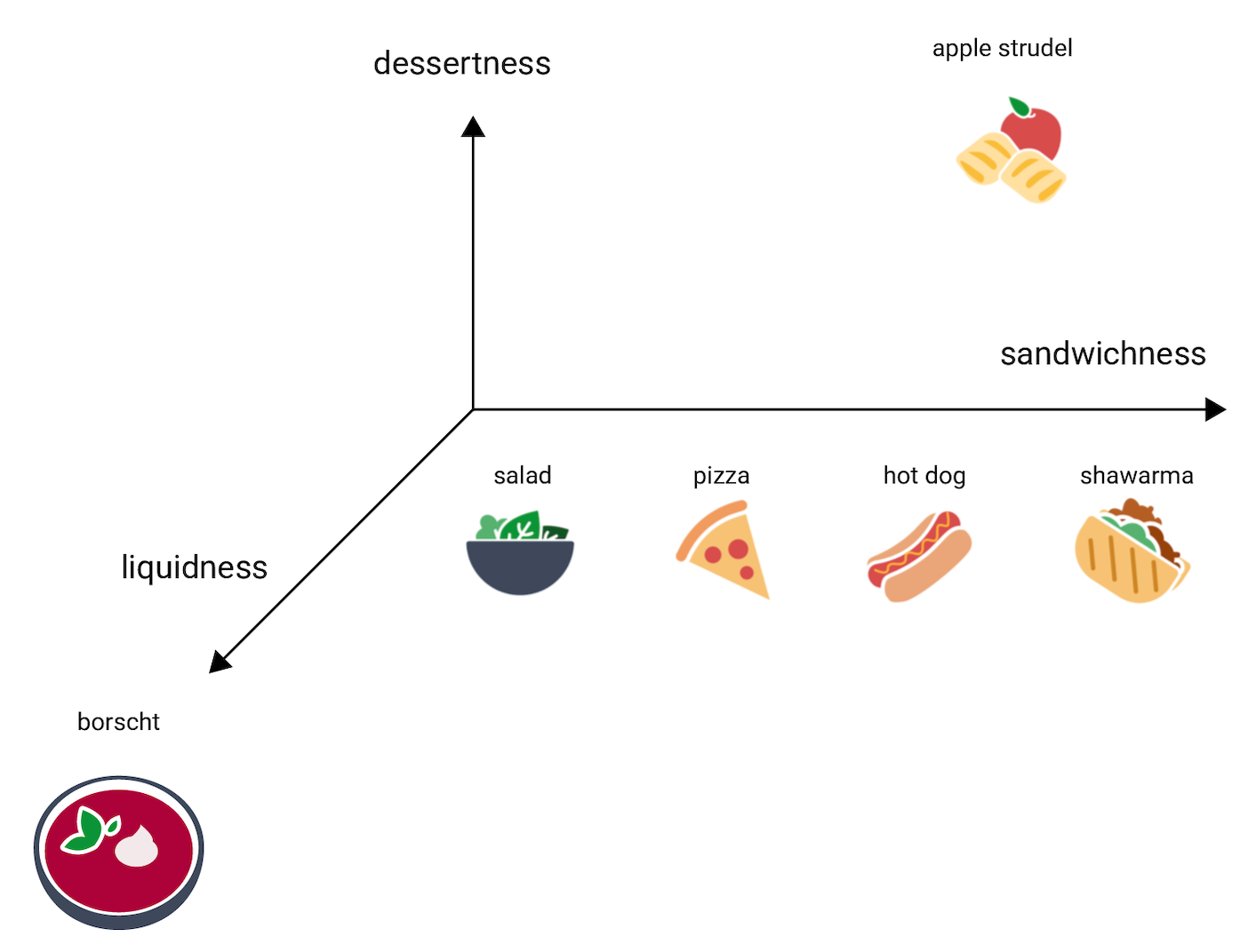
Now consider borscht, which is much more liquid than the other items. This suggests a third dimension, liquidness (how liquid the food is). Adding that dimension, the items could be visualized in 3D in this way:

Figure 5. Foods plotted by "sandwichness," "dessertness," and "liquidness."

Where in this 3D space would tangyuan go? It's soupy, like borscht, and a sweet dessert, like apple strudel, and most definitely not a sandwich. Here is one possible placement:

Figure 6. Adding tangyuan to the previous image, high on "dessertness" and "liquidness" and low on "sandwichness."

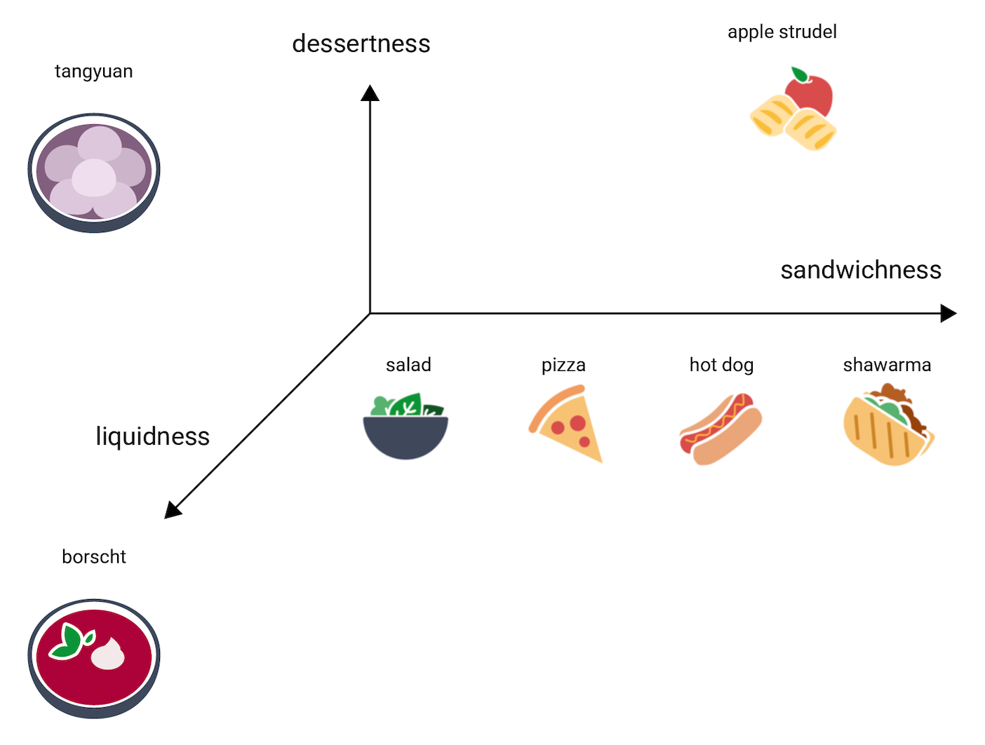
Notice how much information is expressed in these three dimensions. You could imagine additional dimensions, like meatiness or bakedness.

Real-world embedding spaces

As you saw in the food examples above, even a small multi-dimensional space provides the freedom to group semantically similar items together and keep dissimilar items far apart. Position (distance and direction) in the vector space can encode semantics in a good embedding. For example, the following visualizations of real embeddings illustrate the geometrical relationships between the words for a country and its capital. You can see that the distance from "Canada" to "Ottawa" is about the same as the distance from "Turkey" to "Ankara".

Figure 7. Embeddings can produce remarkable analogies.

A meaningful embedding space helps a machine learning model detect patterns during training.

Exercise

In this exercise, you'll use the Embedding Projector tool to visualize a word embedding called word2vec that represents over 70,000 English words numerically in vector space.

Task 1

Perform the following tasks, and then answer the question below.

1. Open the Embedding Projector tool.

2. In the right panel, enter the word atom in the Search field. Then click the word atom from the results below (under 4 matches). Your screen should look like Figure 8.

   

   Figure 8. Embedding projector tool, with the word "atom" added in the Search field (circled in red).

3. Again, in the right panel, click the Isolate 101 points button (above the Search field) to show the nearest 100 words to atom. Your screen should look like Figure 9.

   

   Figure 9. Embedding projector tool, now with "Isolate 101 points" clicked (circled in red).

Now, review the words listed under Nearest points in the original space. How would you describe these words?

Click here for our answer

The majority of the nearest words are words that are commonly associated with the word atom, such as the plural form "atoms," and the words "electron," "molecule," and "nucleus."

Task 2

Perform the following tasks, and then answer the question below:

1. Click the Show All Data button in the right panel to reset the data visualization from Task 1.

2. In the right panel, enter the word uranium in the Search field. Your screen should look like Figure 10.

   

   Figure 10. Embedding projector tool, with the word "uranium" added in the Search field.

Review the words listed under Nearest points in the original space. How are these words different than the nearest words for atom?

Click here for our answer

Uranium refers to a specific radioactive chemical element, and many of the nearest words are other elements, such as zinc, manganese, copper, and aluminum.

Task 3

Perform the following tasks, and then answer the question below:

1. Click the Show All Data button in the right panel to reset the data visualization from Task 2.

2. In the right panel, enter the word orange in the Search field. Your screen should look like Figure 11.

   

   Figure 11. Embedding projector tool, with the word "orange" added in the Search field.

Review the words listed under Nearest points in the original space. What do you notice about the types of words shown here, and the types of words not shown here?

Click here for our answer

Nearly all the nearest words are other colors, such as "yellow," "green," "blue," "purple," and "red." Only one of the nearest words ("juice") refer to the word's other meaning (a citrus fruit). Other fruits you might expect to see, like "apple" and "banana," did not make the list of nearest terms.

This example illustrates one of the key shortcomings of static embeddings like word2vec. All the possible meanings of a word are represented by a single point in vector space, so when you do a similarity analysis for "orange," it's not possible to isolate the nearest points for a specific denotation of the word, such as "orange" (fruit) but not "orange" (color).

Key terms:

• Embedding vector