Page Summary
-
This module introduces linear regression, a statistical method used to predict a label value based on its features.
-
The linear regression model uses an equation (y' = b + w₁x₁ + ...) to represent the relationship between features and the label.
-
During training, the model adjusts its bias (b) and weights (w) to minimize the difference between predicted and actual values.
-
Linear regression can be applied to models with multiple features, each with its own weight, to improve prediction accuracy.
-
Gradient descent and hyperparameter tuning are key techniques used to optimize the performance of a linear regression model.
This module introduces linear regression concepts.
Linear regression is a statistical technique used to find the relationship between variables. In an ML context, linear regression finds the relationship between features and a label.
For example, suppose we want to predict a car's fuel efficiency in miles per gallon based on how heavy the car is, and we have the following dataset:
| Pounds in 1000s (feature) | Miles per gallon (label) |
|---|---|
| 3.5 | 18 |
| 3.69 | 15 |
| 3.44 | 18 |
| 3.43 | 16 |
| 4.34 | 15 |
| 4.42 | 14 |
| 2.37 | 24 |
If we plotted these points, we'd get the following graph:
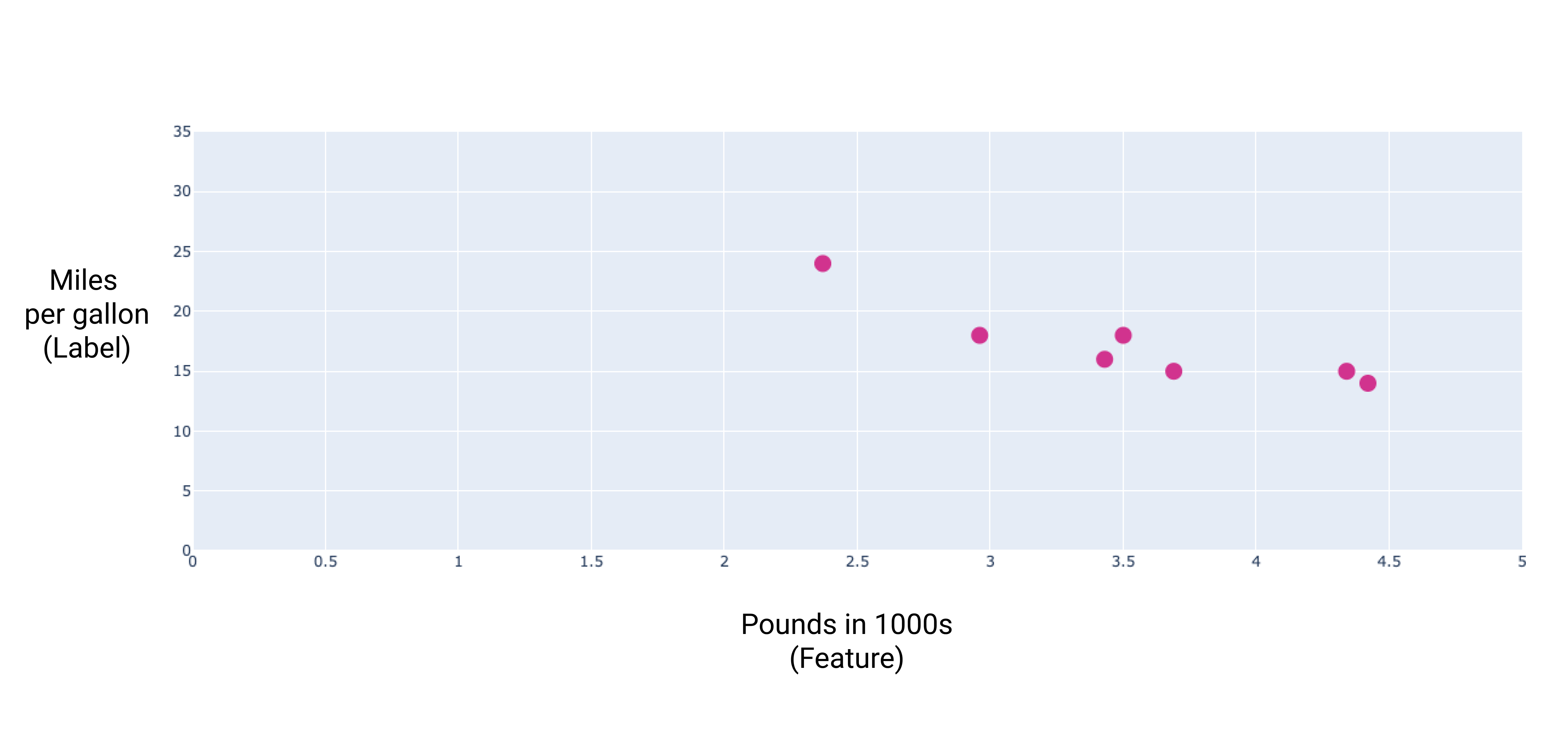
Figure 1. Car heaviness (in pounds) versus miles per gallon rating. As a car gets heavier, its miles per gallon rating generally decreases.
We could create our own model by drawing a best fit line through the points:
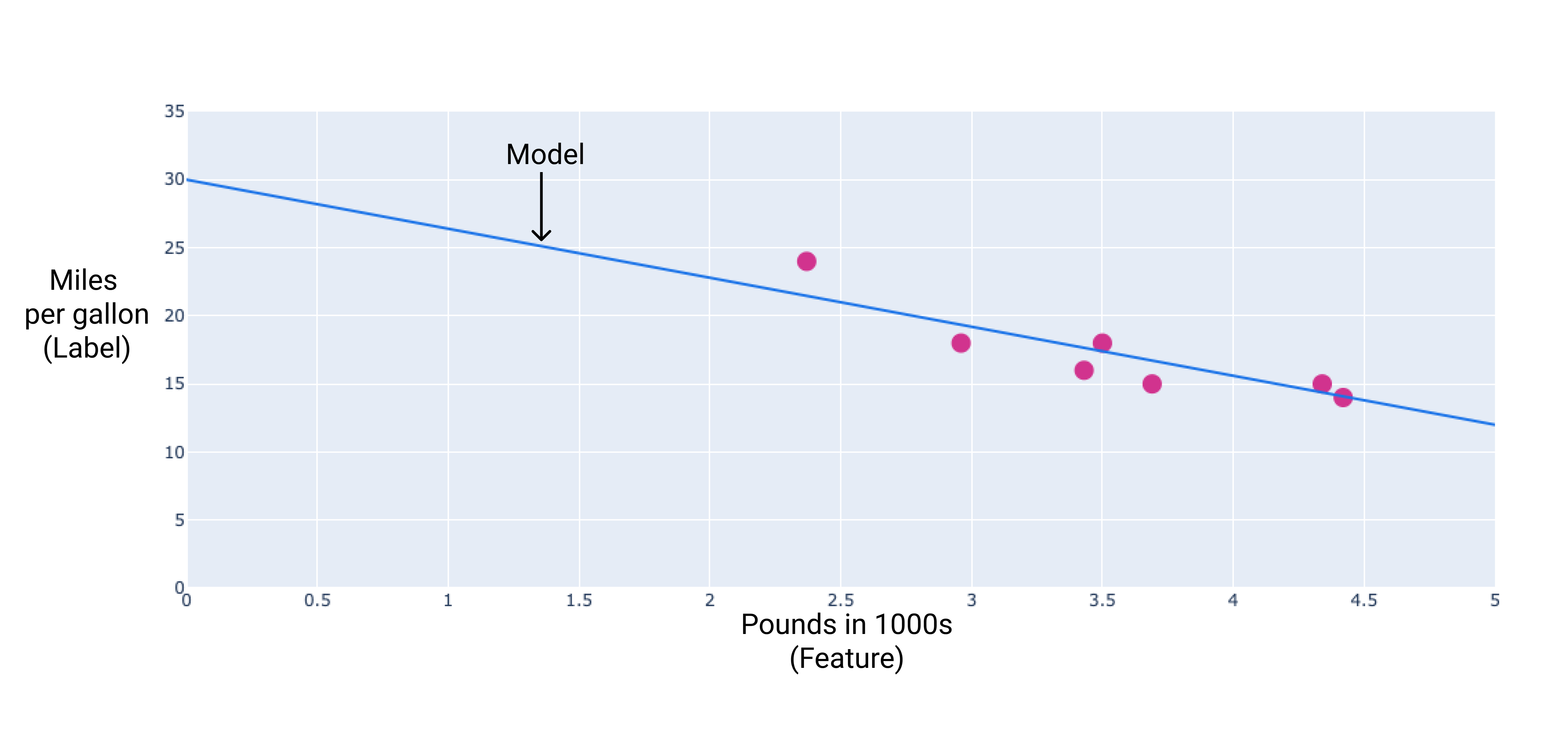
Figure 2. A best fit line drawn through the data from the previous figure.
Linear regression equation
In algebraic terms, the model would be defined as $ y = mx + b $, where
- $ y $ is miles per gallon—the value we want to predict.
- $ m $ is the slope of the line.
- $ x $ is pounds—our input value.
- $ b $ is the y-intercept.
In ML, we write the equation for a linear regression model as follows:
where:
- $ y' $ is the predicted label—the output.
- $ b $ is the bias of the model. Bias is the same concept as the y-intercept in the algebraic equation for a line. In ML, bias is sometimes referred to as $ w_0 $. Bias is a parameter of the model and is calculated during training.
- $ w_1 $ is the weight of the feature. Weight is the same concept as the slope $ m $ in the algebraic equation for a line. Weight is a parameter of the model and is calculated during training.
- $ x_1 $ is a feature—the input.
During training, the model calculates the weight and bias that produce the best model.
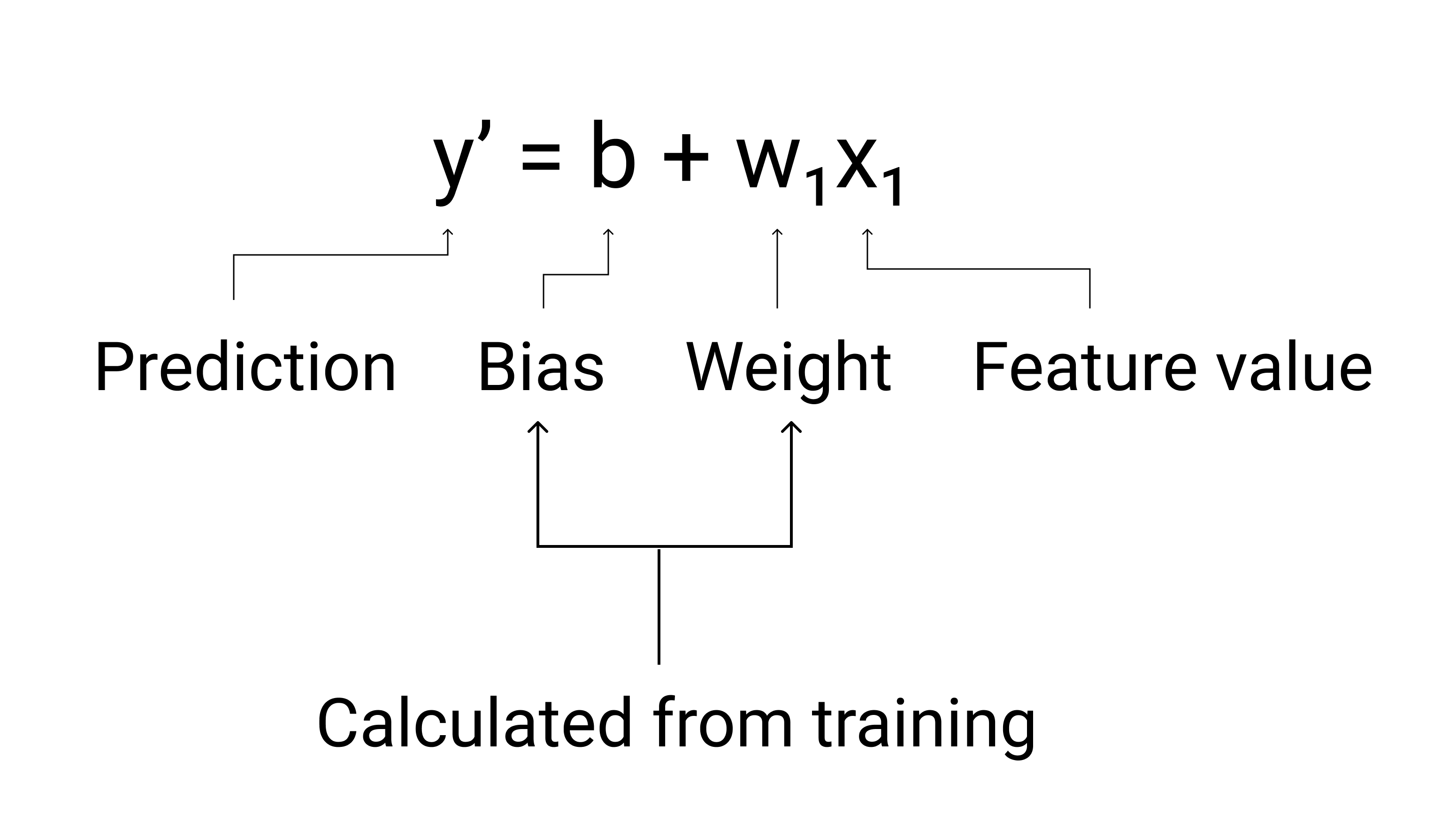
Figure 3. Mathematical representation of a linear model.
In our example, we'd calculate the weight and bias from the line we drew. The bias is 34 (where the line intersects the y-axis), and the weight is –4.6 (the slope of the line). The model would be defined as $ y' = 34 + (-4.6)(x_1) $, and we could use it to make predictions. For instance, using this model, a 4,000-pound car would have a predicted fuel efficiency of 15.6 miles per gallon.
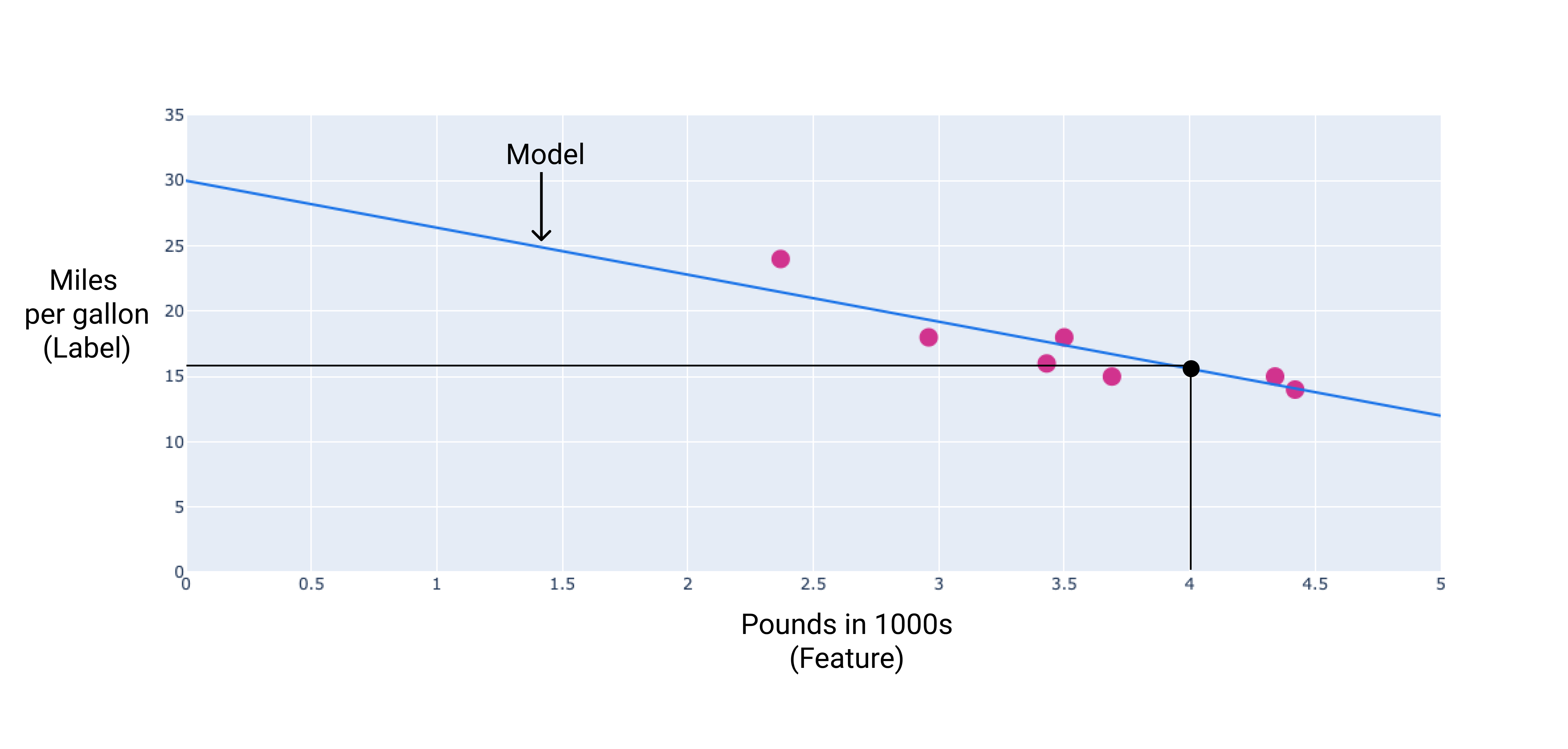
Figure 4. Using the model, a 4,000-pound car has a predicted fuel efficiency of 15.6 miles per gallon.
Models with multiple features
Although the example in this section uses only one feature—the heaviness of the car—a more sophisticated model might rely on multiple features, each having a separate weight ($ w_1 $, $ w_2 $, etc.). For example, a model that relies on five features would be written as follows:
$ y' = b + w_1x_1 + w_2x_2 + w_3x_3 + w_4x_4 + w_5x_5 $
For example, a model that predicts gas mileage could additionally use features such as the following:
- Engine displacement
- Acceleration
- Number of cylinders
- Horsepower
This model would be written as follows:
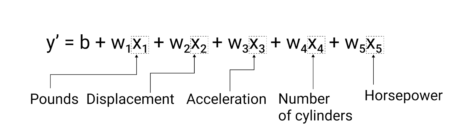
Figure 5. A model with five features to predict a car's miles per gallon rating.
By graphing a couple of these additional features, we can see that they also have a linear relationship to the label, miles per gallon:
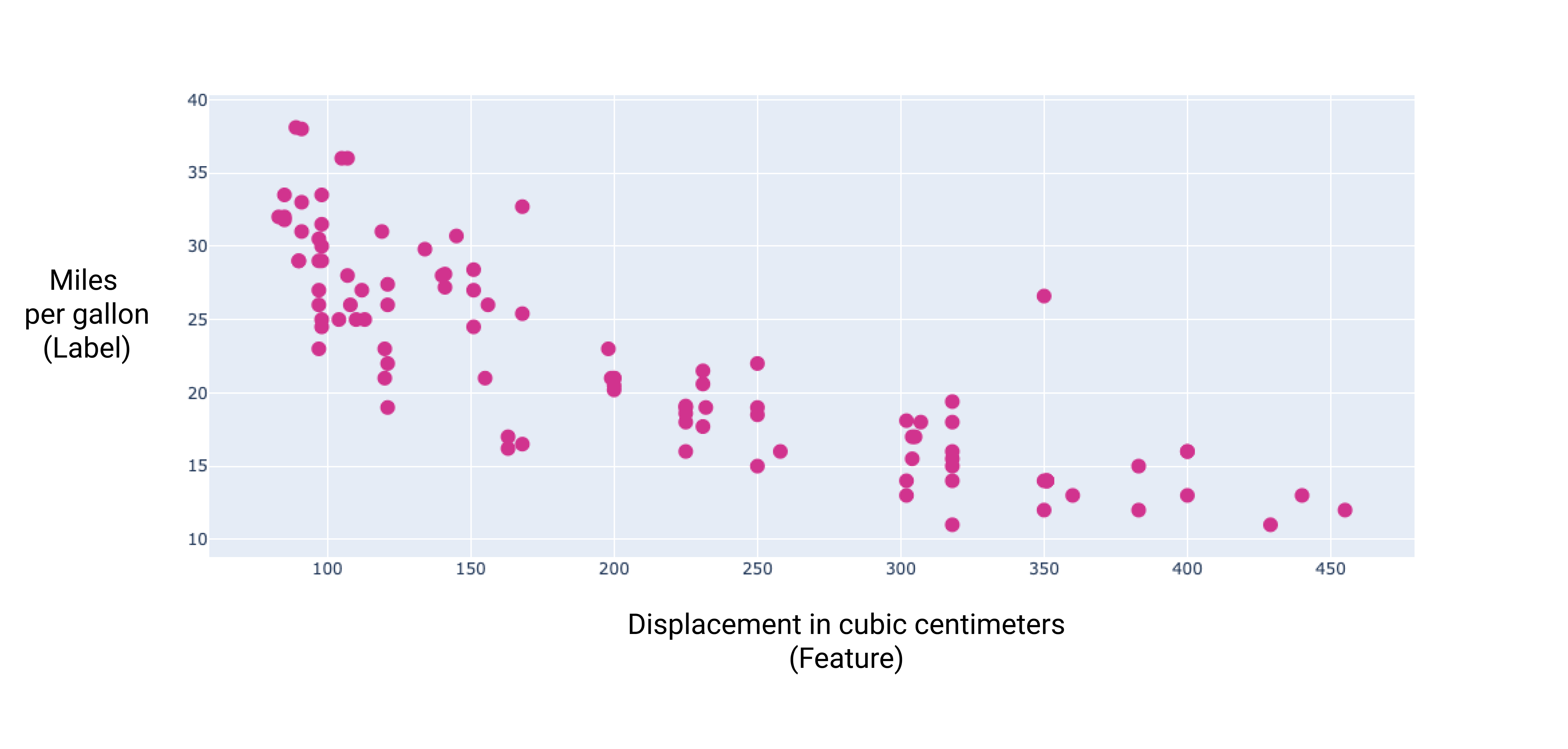
Figure 6. A car's displacement in cubic centimeters and its miles per gallon rating. As a car's engine gets bigger, its miles per gallon rating generally decreases.
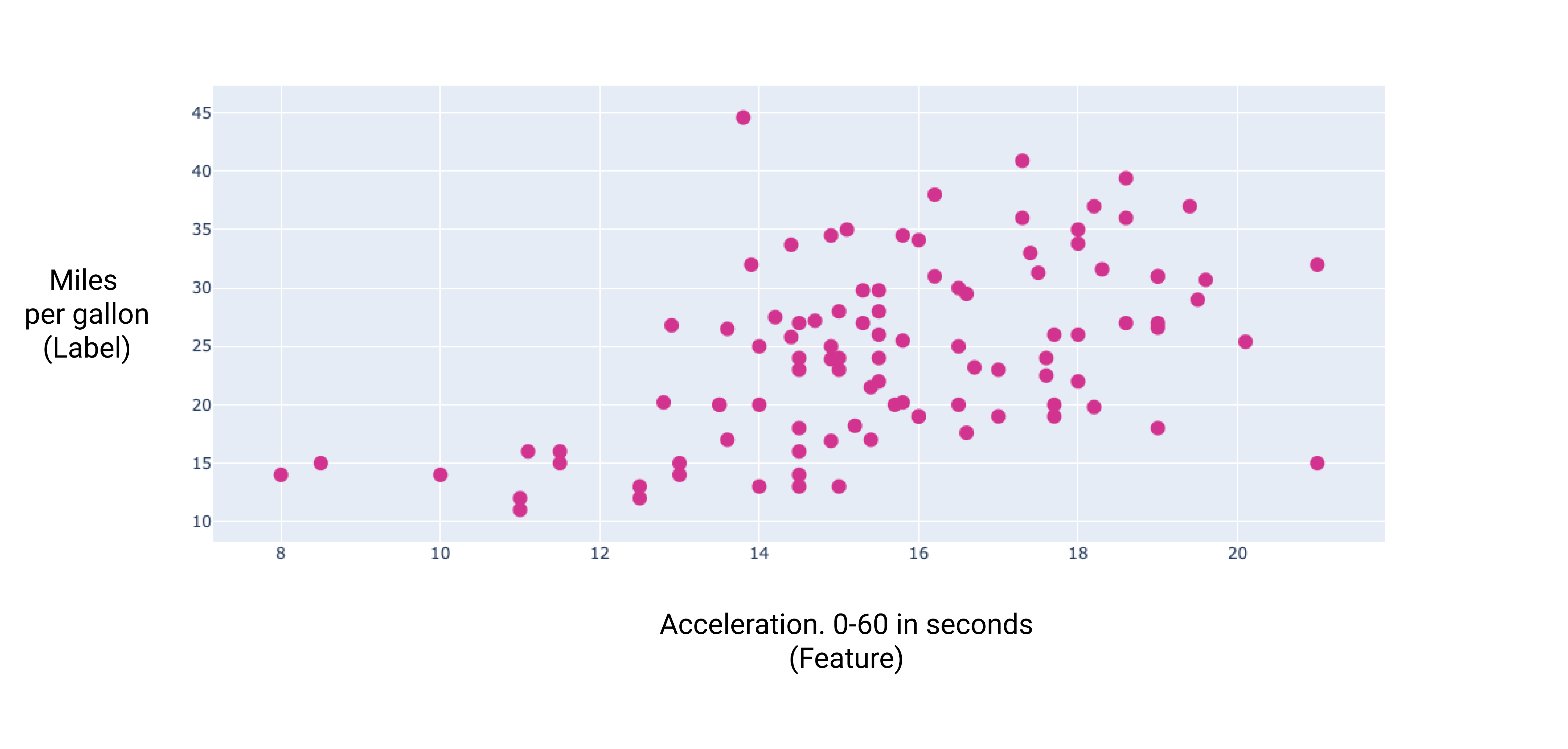
Figure 7. A car's acceleration and its miles per gallon rating. As a car's acceleration takes longer, the miles per gallon rating generally increases.