Resolver un problema con el MIP

En las siguientes secciones, se presenta un ejemplo de un problema de MIP y se muestra cómo resolverlo. Este es el problema:

Maximizar x + 10y sujeto a las siguientes restricciones:

1. x + 7y ≤ 17.5
2. 0 ≤ x ≤ 3.5
3. 0 ≤ y
4. x, y números enteros

Dado que las restricciones son lineales, este es solo un problema de optimización lineal en el que las soluciones deben ser números enteros. En el siguiente gráfico, se muestran los puntos enteros en la región posible para el problema.

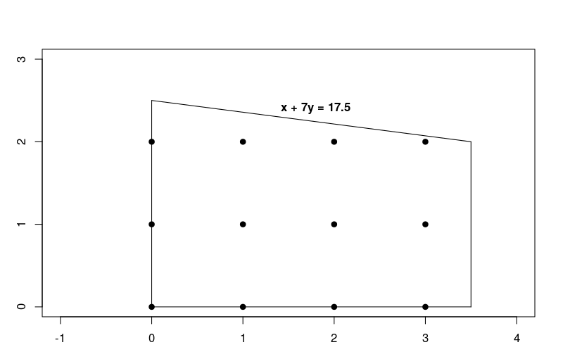
Ten en cuenta que este problema es muy similar al problema de optimización lineal descrito en Cómo resolver un problema de LP, pero, en este caso, se requiere que las soluciones sean números enteros.

Pasos básicos para resolver un problema del MIP

Para resolver un problema del MIP, el programa debe incluir los siguientes pasos:

1. Importa el wrapper de resolución lineal.
2. declara el solucionador de MIP,
3. definir las variables,
4. definir las restricciones,
5. definir el objetivo
6. llamar al solucionador de MIP y
7. mostrar la solución

Solución con MPSolver

En la siguiente sección, se presenta un programa que resuelve el problema con el wrapper MPSolver y un solucionador de MIP.

Nota: Para ejecutar el siguiente programa, debes instalar las herramientas OR.

El solucionador de MIP predeterminado de las herramientas OR es SCIP.

Importa el wrapper de resolución lineal

Importa (o incluye) el wrapper de resolución lineal de las herramientas OR, una interfaz para solucionadores de MIP y solucionadores lineales, como se muestra a continuación.

Python

from ortools.linear_solver import pywraplp

C++

#include <memory>

#include "ortools/linear_solver/linear_solver.h"

Java

import com.google.ortools.Loader;
import com.google.ortools.linearsolver.MPConstraint;
import com.google.ortools.linearsolver.MPObjective;
import com.google.ortools.linearsolver.MPSolver;
import com.google.ortools.linearsolver.MPVariable;

C#

using System;
using Google.OrTools.LinearSolver;

Cómo declarar el solucionador de MIP

En el siguiente código, se declara el solucionador de MIP para el problema. En este ejemplo, se usa el solucionador de problemas de terceros SCIP.

Nota: Si compilas las herramientas OR desde el código fuente y deseas instalar y usar un agente diferente, consulta la guía de guía de instalación para tu plataforma.

Python

# Create the mip solver with the SCIP backend.
solver = pywraplp.Solver.CreateSolver("SAT")
if not solver:
    return

C++

// Create the mip solver with the SCIP backend.
std::unique_ptr<MPSolver> solver(MPSolver::CreateSolver("SCIP"));
if (!solver) {
  LOG(WARNING) << "SCIP solver unavailable.";
  return;
}

Java

// Create the linear solver with the SCIP backend.
MPSolver solver = MPSolver.createSolver("SCIP");
if (solver == null) {
  System.out.println("Could not create solver SCIP");
  return;
}

C#

// Create the linear solver with the SCIP backend.
Solver solver = Solver.CreateSolver("SCIP");
if (solver is null)
{
    return;
}

Define las variables

El siguiente código define las variables en el problema.

Python

infinity = solver.infinity()
# x and y are integer non-negative variables.
x = solver.IntVar(0.0, infinity, "x")
y = solver.IntVar(0.0, infinity, "y")

print("Number of variables =", solver.NumVariables())

C++

const double infinity = solver->infinity();
// x and y are integer non-negative variables.
MPVariable* const x = solver->MakeIntVar(0.0, infinity, "x");
MPVariable* const y = solver->MakeIntVar(0.0, infinity, "y");

LOG(INFO) << "Number of variables = " << solver->NumVariables();

Java

double infinity = java.lang.Double.POSITIVE_INFINITY;
// x and y are integer non-negative variables.
MPVariable x = solver.makeIntVar(0.0, infinity, "x");
MPVariable y = solver.makeIntVar(0.0, infinity, "y");

System.out.println("Number of variables = " + solver.numVariables());

C#

// x and y are integer non-negative variables.
Variable x = solver.MakeIntVar(0.0, double.PositiveInfinity, "x");
Variable y = solver.MakeIntVar(0.0, double.PositiveInfinity, "y");

Console.WriteLine("Number of variables = " + solver.NumVariables());

El programa usa el método MakeIntVar (o una variante, según el lenguaje de programación) para crear variables x y y que acepten valores enteros no negativos.

Define las restricciones

El siguiente código define las restricciones del problema.

Python

# x + 7 * y <= 17.5.
solver.Add(x + 7 * y <= 17.5)

# x <= 3.5.
solver.Add(x <= 3.5)

print("Number of constraints =", solver.NumConstraints())

C++

// x + 7 * y <= 17.5.
MPConstraint* const c0 = solver->MakeRowConstraint(-infinity, 17.5, "c0");
c0->SetCoefficient(x, 1);
c0->SetCoefficient(y, 7);

// x <= 3.5.
MPConstraint* const c1 = solver->MakeRowConstraint(-infinity, 3.5, "c1");
c1->SetCoefficient(x, 1);
c1->SetCoefficient(y, 0);

LOG(INFO) << "Number of constraints = " << solver->NumConstraints();

Java

// x + 7 * y <= 17.5.
MPConstraint c0 = solver.makeConstraint(-infinity, 17.5, "c0");
c0.setCoefficient(x, 1);
c0.setCoefficient(y, 7);

// x <= 3.5.
MPConstraint c1 = solver.makeConstraint(-infinity, 3.5, "c1");
c1.setCoefficient(x, 1);
c1.setCoefficient(y, 0);

System.out.println("Number of constraints = " + solver.numConstraints());

C#

// x + 7 * y <= 17.5.
solver.Add(x + 7 * y <= 17.5);

// x <= 3.5.
solver.Add(x <= 3.5);

Console.WriteLine("Number of constraints = " + solver.NumConstraints());

Define el objetivo

El siguiente código define el elemento objective function del problema.

Python

# Maximize x + 10 * y.
solver.Maximize(x + 10 * y)

C++

// Maximize x + 10 * y.
MPObjective* const objective = solver->MutableObjective();
objective->SetCoefficient(x, 1);
objective->SetCoefficient(y, 10);
objective->SetMaximization();

Java

// Maximize x + 10 * y.
MPObjective objective = solver.objective();
objective.setCoefficient(x, 1);
objective.setCoefficient(y, 10);
objective.setMaximization();

C#

// Maximize x + 10 * y.
solver.Maximize(x + 10 * y);

Cómo llamar al solucionador

El siguiente código llama al solucionador.

Python

print(f"Solving with {solver.SolverVersion()}")
status = solver.Solve()

C++

const MPSolver::ResultStatus result_status = solver->Solve();
// Check that the problem has an optimal solution.
if (result_status != MPSolver::OPTIMAL) {
  LOG(FATAL) << "The problem does not have an optimal solution!";
}

Java

final MPSolver.ResultStatus resultStatus = solver.solve();

C#

Solver.ResultStatus resultStatus = solver.Solve();

Muestra la solución

El siguiente código muestra la solución.

Python

if status == pywraplp.Solver.OPTIMAL:
    print("Solution:")
    print("Objective value =", solver.Objective().Value())
    print("x =", x.solution_value())
    print("y =", y.solution_value())
else:
    print("The problem does not have an optimal solution.")

C++

LOG(INFO) << "Solution:";
LOG(INFO) << "Objective value = " << objective->Value();
LOG(INFO) << "x = " << x->solution_value();
LOG(INFO) << "y = " << y->solution_value();

Java

if (resultStatus == MPSolver.ResultStatus.OPTIMAL) {
  System.out.println("Solution:");
  System.out.println("Objective value = " + objective.value());
  System.out.println("x = " + x.solutionValue());
  System.out.println("y = " + y.solutionValue());
} else {
  System.err.println("The problem does not have an optimal solution!");
}

C#

// Check that the problem has an optimal solution.
if (resultStatus != Solver.ResultStatus.OPTIMAL)
{
    Console.WriteLine("The problem does not have an optimal solution!");
    return;
}
Console.WriteLine("Solution:");
Console.WriteLine("Objective value = " + solver.Objective().Value());
Console.WriteLine("x = " + x.SolutionValue());
Console.WriteLine("y = " + y.SolutionValue());

Esta es la solución al problema.

Number of variables = 2
Number of constraints = 2
Solution:
Objective value = 23
x = 3
y = 2

El valor óptimo de la función objetivo es 23, que se produce en el punto x = 3, y = 2.

Programas completos

Estos son los programas completos.

Python

from ortools.linear_solver import pywraplp


def main():
    # Create the mip solver with the SCIP backend.
    solver = pywraplp.Solver.CreateSolver("SAT")
    if not solver:
        return

    infinity = solver.infinity()
    # x and y are integer non-negative variables.
    x = solver.IntVar(0.0, infinity, "x")
    y = solver.IntVar(0.0, infinity, "y")

    print("Number of variables =", solver.NumVariables())

    # x + 7 * y <= 17.5.
    solver.Add(x + 7 * y <= 17.5)

    # x <= 3.5.
    solver.Add(x <= 3.5)

    print("Number of constraints =", solver.NumConstraints())

    # Maximize x + 10 * y.
    solver.Maximize(x + 10 * y)

    print(f"Solving with {solver.SolverVersion()}")
    status = solver.Solve()

    if status == pywraplp.Solver.OPTIMAL:
        print("Solution:")
        print("Objective value =", solver.Objective().Value())
        print("x =", x.solution_value())
        print("y =", y.solution_value())
    else:
        print("The problem does not have an optimal solution.")

    print("\nAdvanced usage:")
    print(f"Problem solved in {solver.wall_time():d} milliseconds")
    print(f"Problem solved in {solver.iterations():d} iterations")
    print(f"Problem solved in {solver.nodes():d} branch-and-bound nodes")


if __name__ == "__main__":
    main()

C++

#include <memory>

#include "ortools/linear_solver/linear_solver.h"

namespace operations_research {
void SimpleMipProgram() {
  // Create the mip solver with the SCIP backend.
  std::unique_ptr<MPSolver> solver(MPSolver::CreateSolver("SCIP"));
  if (!solver) {
    LOG(WARNING) << "SCIP solver unavailable.";
    return;
  }

  const double infinity = solver->infinity();
  // x and y are integer non-negative variables.
  MPVariable* const x = solver->MakeIntVar(0.0, infinity, "x");
  MPVariable* const y = solver->MakeIntVar(0.0, infinity, "y");

  LOG(INFO) << "Number of variables = " << solver->NumVariables();

  // x + 7 * y <= 17.5.
  MPConstraint* const c0 = solver->MakeRowConstraint(-infinity, 17.5, "c0");
  c0->SetCoefficient(x, 1);
  c0->SetCoefficient(y, 7);

  // x <= 3.5.
  MPConstraint* const c1 = solver->MakeRowConstraint(-infinity, 3.5, "c1");
  c1->SetCoefficient(x, 1);
  c1->SetCoefficient(y, 0);

  LOG(INFO) << "Number of constraints = " << solver->NumConstraints();

  // Maximize x + 10 * y.
  MPObjective* const objective = solver->MutableObjective();
  objective->SetCoefficient(x, 1);
  objective->SetCoefficient(y, 10);
  objective->SetMaximization();

  const MPSolver::ResultStatus result_status = solver->Solve();
  // Check that the problem has an optimal solution.
  if (result_status != MPSolver::OPTIMAL) {
    LOG(FATAL) << "The problem does not have an optimal solution!";
  }

  LOG(INFO) << "Solution:";
  LOG(INFO) << "Objective value = " << objective->Value();
  LOG(INFO) << "x = " << x->solution_value();
  LOG(INFO) << "y = " << y->solution_value();

  LOG(INFO) << "\nAdvanced usage:";
  LOG(INFO) << "Problem solved in " << solver->wall_time() << " milliseconds";
  LOG(INFO) << "Problem solved in " << solver->iterations() << " iterations";
  LOG(INFO) << "Problem solved in " << solver->nodes()
            << " branch-and-bound nodes";
}
}  // namespace operations_research

int main(int argc, char** argv) {
  operations_research::SimpleMipProgram();
  return EXIT_SUCCESS;
}

Java

package com.google.ortools.linearsolver.samples;
import com.google.ortools.Loader;
import com.google.ortools.linearsolver.MPConstraint;
import com.google.ortools.linearsolver.MPObjective;
import com.google.ortools.linearsolver.MPSolver;
import com.google.ortools.linearsolver.MPVariable;

/** Minimal Mixed Integer Programming example to showcase calling the solver. */
public final class SimpleMipProgram {
  public static void main(String[] args) {
    Loader.loadNativeLibraries();
    // Create the linear solver with the SCIP backend.
    MPSolver solver = MPSolver.createSolver("SCIP");
    if (solver == null) {
      System.out.println("Could not create solver SCIP");
      return;
    }

    double infinity = java.lang.Double.POSITIVE_INFINITY;
    // x and y are integer non-negative variables.
    MPVariable x = solver.makeIntVar(0.0, infinity, "x");
    MPVariable y = solver.makeIntVar(0.0, infinity, "y");

    System.out.println("Number of variables = " + solver.numVariables());

    // x + 7 * y <= 17.5.
    MPConstraint c0 = solver.makeConstraint(-infinity, 17.5, "c0");
    c0.setCoefficient(x, 1);
    c0.setCoefficient(y, 7);

    // x <= 3.5.
    MPConstraint c1 = solver.makeConstraint(-infinity, 3.5, "c1");
    c1.setCoefficient(x, 1);
    c1.setCoefficient(y, 0);

    System.out.println("Number of constraints = " + solver.numConstraints());

    // Maximize x + 10 * y.
    MPObjective objective = solver.objective();
    objective.setCoefficient(x, 1);
    objective.setCoefficient(y, 10);
    objective.setMaximization();

    final MPSolver.ResultStatus resultStatus = solver.solve();

    if (resultStatus == MPSolver.ResultStatus.OPTIMAL) {
      System.out.println("Solution:");
      System.out.println("Objective value = " + objective.value());
      System.out.println("x = " + x.solutionValue());
      System.out.println("y = " + y.solutionValue());
    } else {
      System.err.println("The problem does not have an optimal solution!");
    }

    System.out.println("\nAdvanced usage:");
    System.out.println("Problem solved in " + solver.wallTime() + " milliseconds");
    System.out.println("Problem solved in " + solver.iterations() + " iterations");
    System.out.println("Problem solved in " + solver.nodes() + " branch-and-bound nodes");
  }

  private SimpleMipProgram() {}
}

C#

using System;
using Google.OrTools.LinearSolver;

public class SimpleMipProgram
{
    static void Main()
    {
        // Create the linear solver with the SCIP backend.
        Solver solver = Solver.CreateSolver("SCIP");
        if (solver is null)
        {
            return;
        }

        // x and y are integer non-negative variables.
        Variable x = solver.MakeIntVar(0.0, double.PositiveInfinity, "x");
        Variable y = solver.MakeIntVar(0.0, double.PositiveInfinity, "y");

        Console.WriteLine("Number of variables = " + solver.NumVariables());

        // x + 7 * y <= 17.5.
        solver.Add(x + 7 * y <= 17.5);

        // x <= 3.5.
        solver.Add(x <= 3.5);

        Console.WriteLine("Number of constraints = " + solver.NumConstraints());

        // Maximize x + 10 * y.
        solver.Maximize(x + 10 * y);

        Solver.ResultStatus resultStatus = solver.Solve();

        // Check that the problem has an optimal solution.
        if (resultStatus != Solver.ResultStatus.OPTIMAL)
        {
            Console.WriteLine("The problem does not have an optimal solution!");
            return;
        }
        Console.WriteLine("Solution:");
        Console.WriteLine("Objective value = " + solver.Objective().Value());
        Console.WriteLine("x = " + x.SolutionValue());
        Console.WriteLine("y = " + y.SolutionValue());

        Console.WriteLine("\nAdvanced usage:");
        Console.WriteLine("Problem solved in " + solver.WallTime() + " milliseconds");
        Console.WriteLine("Problem solved in " + solver.Iterations() + " iterations");
        Console.WriteLine("Problem solved in " + solver.Nodes() + " branch-and-bound nodes");
    }
}

Comparación de la optimización lineal y de números enteros

Comparemos la solución con el problema de optimización de números enteros que se mostró antes con la solución del problema de optimización lineal correspondiente, en el que se quitan las restricciones de números enteros. Es posible que supongas que la solución para el problema de número entero sería el punto entero en la región posible más cercana a la solución lineal, es decir, el punto x = 0, y = 2. Pero, como verás a continuación, este no es el caso.

Puedes modificar fácilmente el programa de la sección anterior para resolver el problema lineal con los siguientes cambios:

• Cómo reemplazar el solucionador de MIP

  Python

  # Create the mip solver with the SCIP backend.
  solver = pywraplp.Solver.CreateSolver("SAT")
  if not solver:
      return

  C++

  // Create the mip solver with the SCIP backend.
  std::unique_ptr<MPSolver> solver(MPSolver::CreateSolver("SCIP"));
  if (!solver) {
    LOG(WARNING) << "SCIP solver unavailable.";
    return;
  }

  Java

  // Create the linear solver with the SCIP backend.
  MPSolver solver = MPSolver.createSolver("SCIP");
  if (solver == null) {
    System.out.println("Could not create solver SCIP");
    return;
  }

  C#

  // Create the linear solver with the SCIP backend.
  Solver solver = Solver.CreateSolver("SCIP");
  if (solver is null)
  {
      return;
  }

  con el solucionador de problemas de LP

  Python

  # Create the linear solver with the GLOP backend.
  solver = pywraplp.Solver.CreateSolver("GLOP")
  if not solver:
      return

  C++

  // Create the linear solver with the GLOP backend.
  std::unique_ptr<MPSolver> solver(MPSolver::CreateSolver("GLOP"));

  Java

  // Create the linear solver with the GLOP backend.
  MPSolver solver = MPSolver.createSolver("GLOP");
  if (solver == null) {
    System.out.println("Could not create solver SCIP");
    return;
  }

  C#

  // Create the linear solver with the GLOP backend.
  Solver solver = Solver.CreateSolver("GLOP");
  if (solver is null)
  {
      return;
  }

• Reemplaza las variables de números enteros

  Python

  infinity = solver.infinity()
  # x and y are integer non-negative variables.
  x = solver.IntVar(0.0, infinity, "x")
  y = solver.IntVar(0.0, infinity, "y")
  
  print("Number of variables =", solver.NumVariables())

  C++

  const double infinity = solver->infinity();
  // x and y are integer non-negative variables.
  MPVariable* const x = solver->MakeIntVar(0.0, infinity, "x");
  MPVariable* const y = solver->MakeIntVar(0.0, infinity, "y");
  
  LOG(INFO) << "Number of variables = " << solver->NumVariables();

  Java

  double infinity = java.lang.Double.POSITIVE_INFINITY;
  // x and y are integer non-negative variables.
  MPVariable x = solver.makeIntVar(0.0, infinity, "x");
  MPVariable y = solver.makeIntVar(0.0, infinity, "y");
  
  System.out.println("Number of variables = " + solver.numVariables());

  C#

  // x and y are integer non-negative variables.
  Variable x = solver.MakeIntVar(0.0, double.PositiveInfinity, "x");
  Variable y = solver.MakeIntVar(0.0, double.PositiveInfinity, "y");
  
  Console.WriteLine("Number of variables = " + solver.NumVariables());

  con variables continuas

  Python

  infinity = solver.infinity()
  # Create the variables x and y.
  x = solver.NumVar(0.0, infinity, "x")
  y = solver.NumVar(0.0, infinity, "y")
  
  print("Number of variables =", solver.NumVariables())

  C++

  const double infinity = solver->infinity();
  // Create the variables x and y.
  MPVariable* const x = solver->MakeNumVar(0.0, infinity, "x");
  MPVariable* const y = solver->MakeNumVar(0.0, infinity, "y");
  
  LOG(INFO) << "Number of variables = " << solver->NumVariables();

  Java

  double infinity = java.lang.Double.POSITIVE_INFINITY;
  // Create the variables x and y.
  MPVariable x = solver.makeNumVar(0.0, infinity, "x");
  MPVariable y = solver.makeNumVar(0.0, infinity, "y");
  
  System.out.println("Number of variables = " + solver.numVariables());

  C#

  // Create the variables x and y.
  Variable x = solver.MakeNumVar(0.0, double.PositiveInfinity, "x");
  Variable y = solver.MakeNumVar(0.0, double.PositiveInfinity, "y");
  
  Console.WriteLine("Number of variables = " + solver.NumVariables());

Después de realizar estos cambios y volver a ejecutar el programa, obtendrás el siguiente resultado:

Number of variables = 2
Number of constraints = 2
Objective value = 25.000000
x = 0.000000
y = 2.500000

La solución al problema lineal se produce en el punto x = 0, y = 2.5, donde la función objetivo es igual a 25. A continuación, se muestra un gráfico con las soluciones a los problemas lineales y de números enteros.

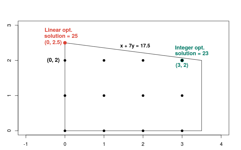
Ten en cuenta que la solución de números enteros no es cercana a la solución lineal, en comparación con la mayoría de los otros puntos de números enteros en la región posible. En general, las soluciones a un problema de optimización lineal y los problemas de optimización de números enteros correspondientes pueden diferir mucho. Debido a esto, los dos tipos de problemas requieren métodos diferentes para su solución.