

 在 Google Colab 中執行
 前往 GitHub 查看原始碼
有許多 ee.Image 方法可產生圖片資料的 RGB 視覺表示法,例如:visualize()、getThumbURL()、getMap()、getMapId() (用於 Colab Folium 地圖顯示) 和 Map.addLayer() (用於程式碼編輯器地圖顯示,不適用於 Python)。根據預設,這些方法會分別將前三個波段指派給紅色、綠色和藍色。預設拉伸是根據波段中的資料類型 (例如浮點數在 [0, 1] 中拉伸,16 位元資料則拉伸至可能值的完整範圍),這可能適合,也可能不適合。如要達到理想的視覺效果,您可以提供視覺化參數:
| 參數 | 說明 | 類型 |
|---|---|---|
| 頻帶 | 以半形逗號分隔的三個波段名稱清單,用於對應至 RGB | list |
| min | 要對應至 0 的值 | 數字或三個數字的清單,每個波段一個 |
| max | 要對應至 255 的值 | 數字或三個數字的清單,每個波段一個 |
| gain | 每個像素值要乘以的值 | 數字或三個數字的清單,每個波段一個 |
| 偏差 | 要新增至各 DN 的值 | 數字或三個數字的清單,每個波段一個 |
| gamma | Gamma 修正係數 | 數字或三個數字的清單,每個波段一個 |
| palette | CSS 樣式顏色字串清單 (僅限單波段圖片) | 以半形逗號分隔的十六進位字串清單 |
| opacity | 圖層的不透明度 (0.0 為完全透明,1.0 為完全不透明) | 數字 |
| 格式 | 「jpg」或「png」 | 字串 |
RGB 複合影像
以下說明如何使用參數,將 Landsat 8 圖片設為假色合成:
程式碼編輯器 (JavaScript)
// Load an image.
var image = ee.Image('LANDSAT/LC08/C02/T1_TOA/LC08_044034_20140318');

// Define the visualization parameters.
var vizParams = {
  bands: ['B5', 'B4', 'B3'],
  min: 0,
  max: 0.5,
  gamma: [0.95, 1.1, 1]
};

// Center the map and display the image.
Map.setCenter(-122.1899, 37.5010, 10); // San Francisco Bay
Map.addLayer(image, vizParams, 'false color composite');
import ee
import geemap.core as geemap
Colab (Python)
# Load an image.
image = ee.Image('LANDSAT/LC08/C02/T1_TOA/LC08_044034_20140318')

# Define the visualization parameters.
image_viz_params = {
    'bands': ['B5', 'B4', 'B3'],
    'min': 0,
    'max': 0.5,
    'gamma': [0.95, 1.1, 1],
}

# Define a map centered on San Francisco Bay.
map_l8 = geemap.Map(center=[37.5010, -122.1899], zoom=10)

# Add the image layer to the map and display it.
map_l8.add_layer(image, image_viz_params, 'false color composite')
display(map_l8)
在本範例中,波段 'B5' 指派給紅色,'B4' 指派給綠色,'B3' 指派給藍色。

調色盤
如要以彩色顯示圖片的單一波段,請使用以 CSS 樣式顏色字串清單表示的色階,設定 palette 參數。(詳情請參閱這份參考資料)。以下範例說明如何使用青色 ('00FFFF') 到藍色 ('0000FF') 的顏色,算繪歸一化差值水體指數 (NDWI) 圖片:
程式碼編輯器 (JavaScript)
// Load an image.
var image = ee.Image('LANDSAT/LC08/C02/T1_TOA/LC08_044034_20140318');

// Create an NDWI image, define visualization parameters and display.
var ndwi = image.normalizedDifference(['B3', 'B5']);
var ndwiViz = {min: 0.5, max: 1, palette: ['00FFFF', '0000FF']};
Map.addLayer(ndwi, ndwiViz, 'NDWI', false);
import ee
import geemap.core as geemap
Colab (Python)
# Load an image.
image = ee.Image('LANDSAT/LC08/C02/T1_TOA/LC08_044034_20140318')

# Create an NDWI image, define visualization parameters and display.
ndwi = image.normalizedDifference(['B3', 'B5'])
ndwi_viz = {'min': 0.5, 'max': 1, 'palette': ['00FFFF', '0000FF']}

# Define a map centered on San Francisco Bay.
map_ndwi = geemap.Map(center=[37.5010, -122.1899], zoom=10)

# Add the image layer to the map and display it.
map_ndwi.add_layer(ndwi, ndwi_viz, 'NDWI')
display(map_ndwi)
在本範例中,請注意 min 和 max 參數會指出應套用調色盤的像素值範圍。中間值則會線性延伸。
另請注意,在程式碼編輯器範例中,show 參數設為 false。因此,圖層新增至地圖時,顯示設定會設為關閉。您隨時可以使用程式碼編輯器地圖右上角的圖層管理工具,再次開啟圖層。

儲存預設調色盤
如要將調色盤儲存在分類圖片上,以免忘記套用,您可以為每個分類波段設定兩個特殊命名的字串圖片屬性。
舉例來說,如果圖片有名為 'landcover' 的波段,且有三個值 0、1 和 2,分別對應「water」、「forest」和「other」類別,您可以設定下列屬性,讓預設視覺效果為每個類別顯示指定顏色 (用於分析的值不會受到影響):
landcover_class_values="0,1,2"landcover_class_palette="0000FF,00FF00,AABBCD"
如要瞭解如何設定資產中繼資料,請參閱「素材資源」頁面。
面具
您可以使用 image.updateMask(),根據遮罩圖片中像素非零的位置,設定個別像素的不透明度。遮罩中等於零的像素會從計算中排除,且不透明度會設為 0 以供顯示。以下範例使用 NDWI 門檻 (如要瞭解門檻,請參閱關係運算一節),更新先前建立的 NDWI 圖層遮罩:
程式碼編輯器 (JavaScript)
// Mask the non-watery parts of the image, where NDWI < 0.4.
var ndwiMasked = ndwi.updateMask(ndwi.gte(0.4));
Map.addLayer(ndwiMasked, ndwiViz, 'NDWI masked');
import ee
import geemap.core as geemap
Colab (Python)
# Mask the non-watery parts of the image, where NDWI < 0.4.
ndwi_masked = ndwi.updateMask(ndwi.gte(0.4))

# Define a map centered on San Francisco Bay.
map_ndwi_masked = geemap.Map(center=[37.5010, -122.1899], zoom=10)

# Add the image layer to the map and display it.
map_ndwi_masked.add_layer(ndwi_masked, ndwi_viz, 'NDWI masked')
display(map_ndwi_masked)
視覺化圖片
使用 image.visualize() 方法將圖片轉換為 8 位元 RGB 圖片,以便顯示或匯出。舉例來說,如要將假色合成和 NDWI 轉換為 3 頻帶顯示圖片,請使用:
程式碼編輯器 (JavaScript)
// Create visualization layers.
var imageRGB = image.visualize({bands: ['B5', 'B4', 'B3'], max: 0.5});
var ndwiRGB = ndwiMasked.visualize({
  min: 0.5,
  max: 1,
  palette: ['00FFFF', '0000FF']
});
import ee
import geemap.core as geemap
Colab (Python)
image_rgb = image.visualize(bands=['B5', 'B4', 'B3'], max=0.5)
ndwi_rgb = ndwi_masked.visualize(min=0.5, max=1, palette=['00FFFF', '0000FF'])
馬賽克
您可以使用遮罩和 imageCollection.mosaic() (如要瞭解鑲嵌,請參閱「鑲嵌」一節),達到各種製圖效果。mosaic() 方法會根據輸入集合中的順序,在輸出圖片中算繪圖層。以下範例使用 mosaic() 結合遮罩 NDWI 和假色合成,並取得新的視覺化:
程式碼編輯器 (JavaScript)
// Mosaic the visualization layers and display (or export).
var mosaic = ee.ImageCollection([imageRGB, ndwiRGB]).mosaic();
Map.addLayer(mosaic, {}, 'mosaic');
import ee
import geemap.core as geemap
Colab (Python)
# Mosaic the visualization layers and display (or export).
mosaic = ee.ImageCollection([image_rgb, ndwi_rgb]).mosaic()

# Define a map centered on San Francisco Bay.
map_mosaic = geemap.Map(center=[37.5010, -122.1899], zoom=10)

# Add the image layer to the map and display it.
map_mosaic.add_layer(mosaic, None, 'mosaic')
display(map_mosaic)
在這個範例中,請注意,系統會將兩個視覺化圖片的清單提供給 ImageCollection 建構函式。清單順序會決定圖片在地圖上的算繪順序。

剪輯片段
image.clip() 方法可用於達到製圖效果。以下範例會將先前建立的馬賽克剪輯至舊金山市周圍的任意緩衝區:
程式碼編輯器 (JavaScript)
// Create a circle by drawing a 20000 meter buffer around a point.
var roi = ee.Geometry.Point([-122.4481, 37.7599]).buffer(20000);

// Display a clipped version of the mosaic.
Map.addLayer(mosaic.clip(roi), null, 'mosaic clipped');
import ee
import geemap.core as geemap
Colab (Python)
# Create a circle by drawing a 20000 meter buffer around a point.
roi = ee.Geometry.Point([-122.4481, 37.7599]).buffer(20000)
mosaic_clipped = mosaic.clip(roi)

# Define a map centered on San Francisco.
map_mosaic_clipped = geemap.Map(center=[37.7599, -122.4481], zoom=10)

# Add the image layer to the map and display it.
map_mosaic_clipped.add_layer(mosaic_clipped, None, 'mosaic clipped')
display(map_mosaic_clipped)
在上述範例中,請注意座標會提供給 Geometry 建構函式,且緩衝區長度指定為 20,000 公尺。如要進一步瞭解幾何圖形,請參閱幾何圖形頁面。

轉譯類別地圖
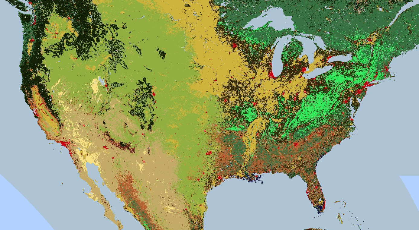
調色盤也適用於轉譯離散值地圖,例如土地覆蓋地圖。
如果有多個類別,請使用調色盤為每個類別提供不同的顏色。(image.remap() 方法在這種情況下可能很有用,可將任意標籤轉換為連續整數)。以下範例使用調色盤算繪土地覆蓋類別:
程式碼編輯器 (JavaScript)
// Load 2012 MODIS land cover and select the IGBP classification.
var cover = ee.Image('MODIS/061/MCD12Q1/2012_01_01')
  .select('LC_Type1');

// Define a palette for the 17 distinct land cover classes.
var igbpPalette = [
  '152106', '225129', '369b47', '30eb5b', '387242', // forest
  '6a2325', 'c3aa69', 'b76031', 'd9903d', '91af40',  // shrub, grass
  '111149', // wetlands
  'cdb33b', // croplands
  'cc0013', // urban
  '33280d', // crop mosaic
  'd7cdcc', // snow and ice
  'f7e084', // barren
  'aec3d4'  // water
];

// Specify the min and max labels and the color palette matching the labels.
Map.setCenter(-99.229, 40.413, 5);
Map.addLayer(cover,
             {min: 1, max: 17, palette: igbpPalette},
             'IGBP classification');
import ee
import geemap.core as geemap
Colab (Python)
# Load 2012 MODIS land cover and select the IGBP classification.
cover = ee.Image('MODIS/061/MCD12Q1/2012_01_01').select('LC_Type1')

# Define a palette for the 17 distinct land cover classes.
igbp_palette = [
    '152106',
    '225129',
    '369b47',
    '30eb5b',
    '387242',  # forest
    '6a2325',
    'c3aa69',
    'b76031',
    'd9903d',
    '91af40',  # shrub, grass
    '111149',  # wetlands
    'cdb33b',  # croplands
    'cc0013',  # urban
    '33280d',  # crop mosaic
    'd7cdcc',  # snow and ice
    'f7e084',  # barren
    'aec3d4',  # water
]

# Define a map centered on the United States.
map_palette = geemap.Map(center=[40.413, -99.229], zoom=5)

# Add the image layer to the map and display it. Specify the min and max labels
# and the color palette matching the labels.
map_palette.add_layer(
    cover, {'min': 1, 'max': 17, 'palette': igbp_palette}, 'IGBP classes'
)
display(map_palette)
樣式化圖層描述元
您可以使用樣式圖層描述元 (SLD) 轉譯圖像以供顯示。向 image.sldStyle() 提供圖片符號和著色的 XML 說明,特別是 RasterSymbolizer 元素。如要進一步瞭解 RasterSymbolizer 元素,請參閱這篇文章。舉例來說,如要使用 SLD 算繪「算繪分類地圖」一節所述的土地覆蓋地圖,請使用:
程式碼編輯器 (JavaScript)
var cover = ee.Image('MODIS/061/MCD12Q1/2012_01_01').select('LC_Type1');

// Define an SLD style of discrete intervals to apply to the image.
var sld_intervals =
'<RasterSymbolizer>' +
  '<ColorMap type="intervals" extended="false">' +
    '<ColorMapEntry color="#152106" quantity="1" label="Evergreen Needleleaf Forest"/>' +
    '<ColorMapEntry color="#225129" quantity="2" label="Evergreen Broadleaf Forest"/>' +
    '<ColorMapEntry color="#369b47" quantity="3" label="Deciduous Needleleaf Forest"/>' +
    '<ColorMapEntry color="#30eb5b" quantity="4" label="Deciduous Broadleaf Forest"/>' +
    '<ColorMapEntry color="#387242" quantity="5" label="Mixed Deciduous Forest"/>' +
    '<ColorMapEntry color="#6a2325" quantity="6" label="Closed Shrubland"/>' +
    '<ColorMapEntry color="#c3aa69" quantity="7" label="Open Shrubland"/>' +
    '<ColorMapEntry color="#b76031" quantity="8" label="Woody Savanna"/>' +
    '<ColorMapEntry color="#d9903d" quantity="9" label="Savanna"/>' +
    '<ColorMapEntry color="#91af40" quantity="10" label="Grassland"/>' +
    '<ColorMapEntry color="#111149" quantity="11" label="Permanent Wetland"/>' +
    '<ColorMapEntry color="#cdb33b" quantity="12" label="Cropland"/>' +
    '<ColorMapEntry color="#cc0013" quantity="13" label="Urban"/>' +
    '<ColorMapEntry color="#33280d" quantity="14" label="Crop, Natural Veg. Mosaic"/>' +
    '<ColorMapEntry color="#d7cdcc" quantity="15" label="Permanent Snow, Ice"/>' +
    '<ColorMapEntry color="#f7e084" quantity="16" label="Barren, Desert"/>' +
    '<ColorMapEntry color="#aec3d4" quantity="17" label="Water"/>' +
  '</ColorMap>' +
'</RasterSymbolizer>';
Map.addLayer(cover.sldStyle(sld_intervals), {}, 'IGBP classification styled');
import ee
import geemap.core as geemap
Colab (Python)
cover = ee.Image('MODIS/061/MCD12Q1/2012_01_01').select('LC_Type1')

# Define an SLD style of discrete intervals to apply to the image.
sld_intervals = """
<RasterSymbolizer>
  <ColorMap  type="intervals" extended="false" >
    <ColorMapEntry color="#152106" quantity="1" label="Evergreen Needleleaf Forest"/>
    <ColorMapEntry color="#225129" quantity="2" label="Evergreen Broadleaf Forest"/>
    <ColorMapEntry color="#369b47" quantity="3" label="Deciduous Needleleaf Forest"/>
    <ColorMapEntry color="#30eb5b" quantity="4" label="Deciduous Broadleaf Forest"/>
    <ColorMapEntry color="#387242" quantity="5" label="Mixed Deciduous Forest"/>
    <ColorMapEntry color="#6a2325" quantity="6" label="Closed Shrubland"/>
    <ColorMapEntry color="#c3aa69" quantity="7" label="Open Shrubland"/>
    <ColorMapEntry color="#b76031" quantity="8" label="Woody Savanna"/>
    <ColorMapEntry color="#d9903d" quantity="9" label="Savanna"/>
    <ColorMapEntry color="#91af40" quantity="10" label="Grassland"/>
    <ColorMapEntry color="#111149" quantity="11" label="Permanent Wetland"/>
    <ColorMapEntry color="#cdb33b" quantity="12" label="Cropland"/>
    <ColorMapEntry color="#cc0013" quantity="13" label="Urban"/>
    <ColorMapEntry color="#33280d" quantity="14" label="Crop, Natural Veg. Mosaic"/>
    <ColorMapEntry color="#d7cdcc" quantity="15" label="Permanent Snow, Ice"/>
    <ColorMapEntry color="#f7e084" quantity="16" label="Barren, Desert"/>
    <ColorMapEntry color="#aec3d4" quantity="17" label="Water"/>
  </ColorMap>
</RasterSymbolizer>"""

# Apply the SLD style to the image.
cover_sld = cover.sldStyle(sld_intervals)

# Define a map centered on the United States.
map_sld_categorical = geemap.Map(center=[40.413, -99.229], zoom=5)

# Add the image layer to the map and display it.
map_sld_categorical.add_layer(cover_sld, None, 'IGBP classes styled')
display(map_sld_categorical)
如要建立含有色階的視覺化圖片,請將 ColorMap 的類型設為「ramp」。以下範例比較了用於算繪 DEM 的「interval」和「ramp」類型:
程式碼編輯器 (JavaScript)
// Load SRTM Digital Elevation Model data.
var image = ee.Image('CGIAR/SRTM90_V4');

// Define an SLD style of discrete intervals to apply to the image. Use the
// opacity keyword to set pixels less than 0 as completely transparent. Pixels
// with values greater than or equal to the final entry quantity are set to
// fully transparent by default.
var sld_intervals =
  '<RasterSymbolizer>' +
    '<ColorMap type="intervals" extended="false" >' +
      '<ColorMapEntry color="#0000ff" quantity="0" label="0 ﹤ x" opacity="0" />' +
      '<ColorMapEntry color="#00ff00" quantity="100" label="0 ≤ x ﹤ 100" />' +
      '<ColorMapEntry color="#007f30" quantity="200" label="100 ≤ x ﹤ 200" />' +
      '<ColorMapEntry color="#30b855" quantity="300" label="200 ≤ x ﹤ 300" />' +
      '<ColorMapEntry color="#ff0000" quantity="400" label="300 ≤ x ﹤ 400" />' +
      '<ColorMapEntry color="#ffff00" quantity="900" label="400 ≤ x ﹤ 900" />' +
    '</ColorMap>' +
  '</RasterSymbolizer>';

// Define an sld style color ramp to apply to the image.
var sld_ramp =
  '<RasterSymbolizer>' +
    '<ColorMap type="ramp" extended="false" >' +
      '<ColorMapEntry color="#0000ff" quantity="0" label="0"/>' +
      '<ColorMapEntry color="#00ff00" quantity="100" label="100" />' +
      '<ColorMapEntry color="#007f30" quantity="200" label="200" />' +
      '<ColorMapEntry color="#30b855" quantity="300" label="300" />' +
      '<ColorMapEntry color="#ff0000" quantity="400" label="400" />' +
      '<ColorMapEntry color="#ffff00" quantity="500" label="500" />' +
    '</ColorMap>' +
  '</RasterSymbolizer>';

// Add the image to the map using both the color ramp and interval schemes.
Map.setCenter(-76.8054, 42.0289, 8);
Map.addLayer(image.sldStyle(sld_intervals), {}, 'SLD intervals');
Map.addLayer(image.sldStyle(sld_ramp), {}, 'SLD ramp');
import ee
import geemap.core as geemap
Colab (Python)
# Load SRTM Digital Elevation Model data.
image = ee.Image('CGIAR/SRTM90_V4')

# Define an SLD style of discrete intervals to apply to the image.
sld_intervals = """
    <RasterSymbolizer>
      <ColorMap type="intervals" extended="false" >
        <ColorMapEntry color="#0000ff" quantity="0" label="0"/>
        <ColorMapEntry color="#00ff00" quantity="100" label="1-100" />
        <ColorMapEntry color="#007f30" quantity="200" label="110-200" />
        <ColorMapEntry color="#30b855" quantity="300" label="210-300" />
        <ColorMapEntry color="#ff0000" quantity="400" label="310-400" />
        <ColorMapEntry color="#ffff00" quantity="1000" label="410-1000" />
      </ColorMap>
    </RasterSymbolizer>"""

# Define an sld style color ramp to apply to the image.
sld_ramp = """
    <RasterSymbolizer>
      <ColorMap type="ramp" extended="false" >
        <ColorMapEntry color="#0000ff" quantity="0" label="0"/>
        <ColorMapEntry color="#00ff00" quantity="100" label="100" />
        <ColorMapEntry color="#007f30" quantity="200" label="200" />
        <ColorMapEntry color="#30b855" quantity="300" label="300" />
        <ColorMapEntry color="#ff0000" quantity="400" label="400" />
        <ColorMapEntry color="#ffff00" quantity="500" label="500" />
      </ColorMap>
    </RasterSymbolizer>"""

# Define a map centered on the United States.
map_sld_interval = geemap.Map(center=[40.413, -99.229], zoom=5)

# Add the image layers to the map and display it.
map_sld_interval.add_layer(
    image.sldStyle(sld_intervals), None, 'SLD intervals'
)
map_sld_interval.add_layer(image.sldStyle(sld_ramp), None, 'SLD ramp')
display(map_sld_interval)
SLD 也可用於延伸像素值,改善連續資料的視覺效果。舉例來說,下列程式碼會比較任意線性拉伸與最小-最大「正規化」和「直方圖」等化的結果:
程式碼編輯器 (JavaScript)
// Load a Landsat 8 raw image.
var image = ee.Image('LANDSAT/LC08/C02/T1/LC08_044034_20140318');

// Define a RasterSymbolizer element with '_enhance_' for a placeholder.
var template_sld =
  '<RasterSymbolizer>' +
    '<ContrastEnhancement><_enhance_/></ContrastEnhancement>' +
    '<ChannelSelection>' +
      '<RedChannel>' +
        '<SourceChannelName>B5</SourceChannelName>' +
      '</RedChannel>' +
      '<GreenChannel>' +
        '<SourceChannelName>B4</SourceChannelName>' +
      '</GreenChannel>' +
      '<BlueChannel>' +
        '<SourceChannelName>B3</SourceChannelName>' +
      '</BlueChannel>' +
    '</ChannelSelection>' +
  '</RasterSymbolizer>';

// Get SLDs with different enhancements.
var equalize_sld = template_sld.replace('_enhance_', 'Histogram');
var normalize_sld = template_sld.replace('_enhance_', 'Normalize');

// Display the results.
Map.centerObject(image, 10);
Map.addLayer(image, {bands: ['B5', 'B4', 'B3'], min: 0, max: 15000}, 'Linear');
Map.addLayer(image.sldStyle(equalize_sld), {}, 'Equalized');
Map.addLayer(image.sldStyle(normalize_sld), {}, 'Normalized');
import ee
import geemap.core as geemap
Colab (Python)
# Load a Landsat 8 raw image.
image = ee.Image('LANDSAT/LC08/C02/T1/LC08_044034_20140318')

# Define a RasterSymbolizer element with '_enhance_' for a placeholder.
template_sld = """
<RasterSymbolizer>
  <ContrastEnhancement><_enhance_/></ContrastEnhancement>
  <ChannelSelection>
    <RedChannel>
      <SourceChannelName>B5</SourceChannelName>
    </RedChannel>
    <GreenChannel>
      <SourceChannelName>B4</SourceChannelName>
    </GreenChannel>
    <BlueChannel>
      <SourceChannelName>B3</SourceChannelName>
    </BlueChannel>
  </ChannelSelection>
</RasterSymbolizer>"""

# Get SLDs with different enhancements.
equalize_sld = template_sld.replace('_enhance_', 'Histogram')
normalize_sld = template_sld.replace('_enhance_', 'Normalize')

# Define a map centered on San Francisco Bay.
map_sld_continuous = geemap.Map(center=[37.5010, -122.1899], zoom=10)

# Add the image layers to the map and display it.
map_sld_continuous.add_layer(
    image, {'bands': ['B5', 'B4', 'B3'], 'min': 0, 'max': 15000}, 'Linear'
)
map_sld_continuous.add_layer(image.sldStyle(equalize_sld), None, 'Equalized')
map_sld_continuous.add_layer(
    image.sldStyle(normalize_sld), None, 'Normalized'
)
display(map_sld_continuous)
在 Earth Engine 中使用 SLD 的注意事項:
- 支援 OGC SLD 1.0 和 OGC SE 1.1。
- 傳入的 XML 文件可以是完整文件,也可以只包含 RasterSymbolizer 元素和子元素。
- 您可以依 Earth Engine 名稱或索引 (「1」、「2」等) 選取波段。
- 浮點圖像不支援直方圖和正規化對比度延展機制。
- 只有在不透明度為 0.0 (透明) 時,系統才會考量不透明度。非零的不透明度值會視為完全不透明。
- 系統目前會忽略 OverlapBehavior 定義。
- 目前不支援 ShadedRelief 機制。
- 目前不支援 ImageOutline 機制。
- 系統會忽略 Geometry 元素。
- 如果要求直方圖等化或正規化,輸出圖片會包含 histogram_bandname 中繼資料。
縮圖圖片
使用 ee.Image.getThumbURL() 方法,為 ee.Image 物件產生 PNG 或 JPEG 縮圖。如果運算式結尾呼叫 getThumbURL(),輸出結果會是網址。造訪網址後,Earth Engine 伺服器會立即產生要求的縮圖。處理完成後,圖片會顯示在瀏覽器中。只要在圖片上按一下滑鼠右鍵,從內容選單中選取適當選項,即可下載。
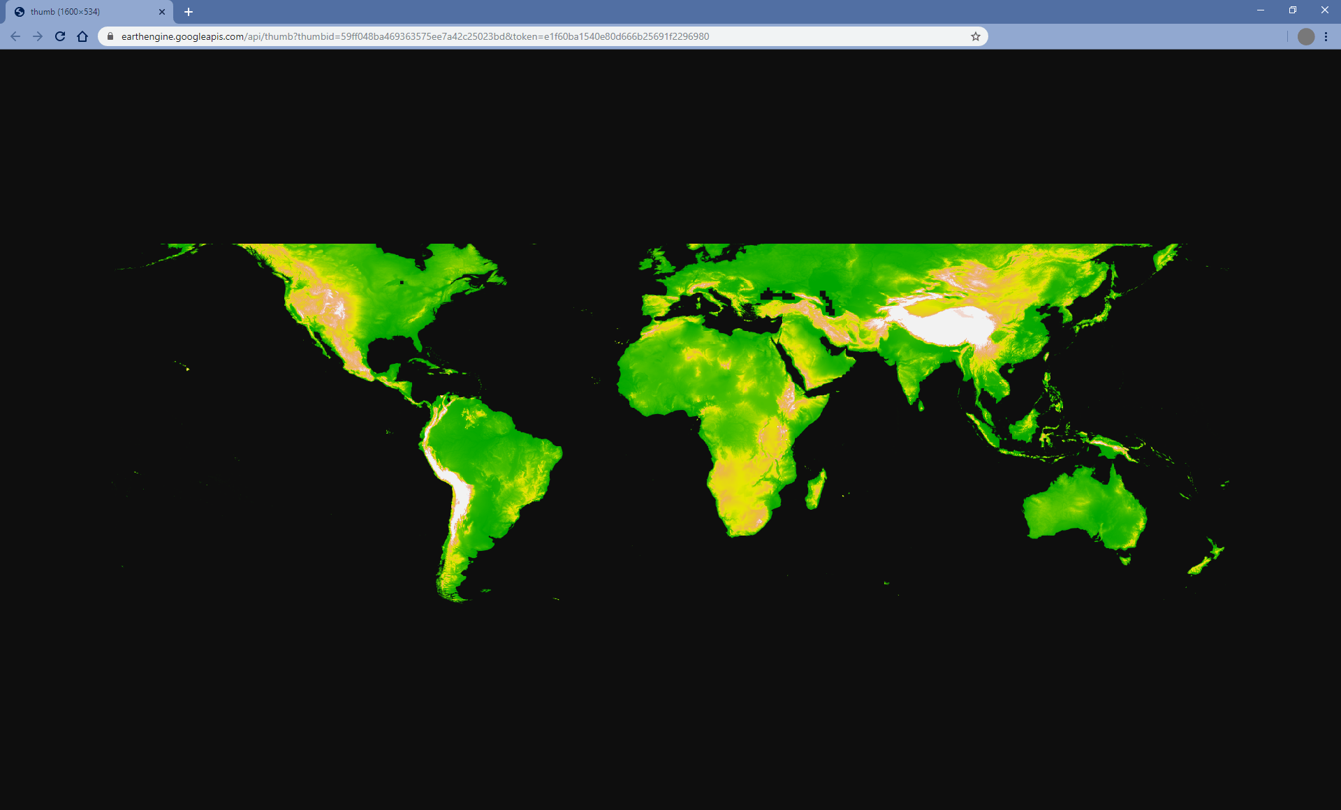
getThumbURL() 方法包含參數,詳情請參閱上方的視覺化參數表。此外,它也接受選用的 dimensions、region 和 crs 引數,用於控制縮圖的空間範圍、大小和顯示投影。
| 參數 | 說明 | 類型 |
|---|---|---|
| 維度 | 縮圖尺寸 (以像素為單位)。如果提供單一整數,則會定義圖片較大顯示比例維度的大小,並按比例縮放較小的維度。預設為 512 像素,用於較大的圖片長寬尺寸。 | 單一整數或字串,格式為: 'WIDTHxHEIGHT' |
| region | 要算繪的圖片地理空間區域。預設為整張圖片,或所提供幾何圖形的邊界。 | GeoJSON 或至少三個點座標的 2D 清單,用於定義線性環 |
| crs | 目標投影,例如「EPSG:3857」。預設為 WGS84 ('EPSG:4326')。 | 字串 |
| 格式 | 將縮圖格式定義為 PNG 或 JPEG。預設 PNG 格式會以 RGBA 實作,其中 Alpha 管道代表有效和無效像素,由圖片的 mask() 定義。無效像素會顯示為透明。選用的 JPEG 格式會以 RGB 實作,其中無效的圖片像素會在 RGB 色彩通道中填入零。 |
字串;「png」或「jpg」 |
除非提供 palette 引數,否則單一波段圖片預設會顯示為灰階。除非提供 bands 引數,否則多頻帶圖片預設會以 RGB 視覺化呈現前三個頻帶。如果只提供兩個波段,第一個波段會對應至紅色,第二個波段會對應至藍色,綠色通道則會填入零。
以下是一系列範例,示範 getThumbURL() 參數引數的各種組合。執行這個指令碼時,點選顯示的網址即可查看縮圖。
程式碼編輯器 (JavaScript)
// Fetch a digital elevation model.
var image = ee.Image('CGIAR/SRTM90_V4');

// Request a default thumbnail of the DEM with defined linear stretch.
// Set masked pixels (ocean) to 1000 so they map as gray.
var thumbnail1 = image.unmask(1000).getThumbURL({
  'min': 0,
  'max': 3000,
  'dimensions': 500,
});
print('Default extent:', thumbnail1);

// Specify region by rectangle, define palette, set larger aspect dimension size.
var thumbnail2 = image.getThumbURL({
  'min': 0,
  'max': 3000,
  'palette': ['00A600','63C600','E6E600','E9BD3A','ECB176','EFC2B3','F2F2F2'],
  'dimensions': 500,
  'region': ee.Geometry.Rectangle([-84.6, -55.9, -32.9, 15.7]),
});
print('Rectangle region and palette:', thumbnail2);

// Specify region by a linear ring and set display CRS as Web Mercator.
var thumbnail3 = image.getThumbURL({
  'min': 0,
  'max': 3000,
  'palette': ['00A600','63C600','E6E600','E9BD3A','ECB176','EFC2B3','F2F2F2'],
  'region': ee.Geometry.LinearRing([[-84.6, 15.7], [-84.6, -55.9], [-32.9, -55.9]]),
  'dimensions': 500,
  'crs': 'EPSG:3857'
});
print('Linear ring region and specified crs', thumbnail3);
import ee
import geemap.core as geemap
Colab (Python)
# Fetch a digital elevation model.
image = ee.Image('CGIAR/SRTM90_V4')

# Request a default thumbnail of the DEM with defined linear stretch.
# Set masked pixels (ocean) to 1000 so they map as gray.
thumbnail_1 = image.unmask(1000).getThumbURL({
    'min': 0,
    'max': 3000,
    'dimensions': 500,
})
print('Default extent:', thumbnail_1)

# Specify region by rectangle, define palette, set larger aspect dimension size.
thumbnail_2 = image.getThumbURL({
    'min': 0,
    'max': 3000,
    'palette': [
        '00A600',
        '63C600',
        'E6E600',
        'E9BD3A',
        'ECB176',
        'EFC2B3',
        'F2F2F2',
    ],
    'dimensions': 500,
    'region': ee.Geometry.Rectangle([-84.6, -55.9, -32.9, 15.7]),
})
print('Rectangle region and palette:', thumbnail_2)

# Specify region by a linear ring and set display CRS as Web Mercator.
thumbnail_3 = image.getThumbURL({
    'min': 0,
    'max': 3000,
    'palette': [
        '00A600',
        '63C600',
        'E6E600',
        'E9BD3A',
        'ECB176',
        'EFC2B3',
        'F2F2F2',
    ],
    'region': ee.Geometry.LinearRing(
        [[-84.6, 15.7], [-84.6, -55.9], [-32.9, -55.9]]
    ),
    'dimensions': 500,
    'crs': 'EPSG:3857',
})
print('Linear ring region and specified crs:', thumbnail_3)