请注意,您可以print()过滤后的集合。您一次最多只能打印 5,000 件物品,因此无法打印整个 l8 系列。执行 print() 方法后,您可以在控制台中检查打印的集合。请注意,当您使用 zippy () 展开 ImageCollection,然后展开 features 的列表时,您会看到一个图片列表,其中的每张图片也可以展开并检查。这是发现单个图片 ID 的一种方法。另一种以更程序化的方式获取用于分析的单个图片的方法是,对集合进行排序,以获取相对于某些元数据属性的最新、最旧或最佳图片。例如,通过检查打印的图片集中的图片对象,您可能会发现一个名为 CLOUD_COVER 的元数据属性。您可以使用该属性获取 2015 年感兴趣区域内云量最少的图片:
代码编辑器 (JavaScript)
// This will sort from least to most cloudy.varsorted=temporalFiltered.sort('CLOUD_COVER');// Get the first (least cloudy) image.varscene=sorted.first();
[null,null,["最后更新时间 (UTC):2025-07-27。"],[[["\u003cp\u003eAn \u003ccode\u003eee.ImageCollection\u003c/code\u003e in Earth Engine represents a set of images, such as all Landsat 8 images, and can be filtered by location and date.\u003c/p\u003e\n"],["\u003cp\u003eIndividual images within a collection can be accessed by sorting based on metadata properties like cloud cover, allowing selection of specific images.\u003c/p\u003e\n"],["\u003cp\u003eDisplaying images requires specifying visualization parameters, like bands for RGB composites and stretching values, for optimal visualization.\u003c/p\u003e\n"],["\u003cp\u003eImage collections can be added to the map, displayed as recent-value composites, showing the most recent pixels and potential cloud cover.\u003c/p\u003e\n"],["\u003cp\u003eEarth Engine's capabilities extend beyond single scenes, enabling large-scale analyses using entire image collections and advanced compositing techniques.\u003c/p\u003e\n"]]],[],null,["# Image Collections\n\nAn image collection refers to a set of Earth Engine images. For example, the collection\nof all Landsat 8 images is an `ee.ImageCollection`. Like the SRTM image\nyou have been working with, image collections also have an ID. As with single images,\nyou can discover the ID of an image collection by searching the\n[Earth Engine data catalog](/earth-engine/datasets) from\nthe Code Editor and looking at the details page of the dataset. For example, search for\n'landsat 8 toa' and click on the first result, which should correspond to the\n[USGS Landsat 8 Collection 1 Tier 1 TOA Reflectance](https://developers.google.com/earth-engine/datasets/catalog/LANDSAT_LC08_C01_T1_TOA) dataset.\nEither import that dataset using the **Import** button and rename it to `l8`, or copy the ID into the\nimage collection constructor:\n\n### Code Editor (JavaScript)\n\n```javascript\nvar l8 = ee.ImageCollection('LANDSAT/LC08/C02/T1_TOA');\n```\n\nFiltering image collections\n---------------------------\n\nIt's worth noting that this collection represents *every* Landsat 8 scene collected,\nall over the Earth. Often it is useful to extract a single image, or subset of images,\non which to test algorithms. The way to limit the collection by time or space is by\nfiltering it. For example, to filter the collection to images that cover a particular\nlocation, first define your area of interest\nwith a point (or line or polygon) using the geometry drawing tools. Pan to your area of\ninterest, hover on the **Geometry Imports** (if you already have one or more\ngeometries defined) and click **+new layer** (if you don't have any imports,\ngo to the next step). Get the point drawing tool\n() and make a point in your area of\ninterest. Name the import `point`. Now, filter the `l8` collection\nto get *only* the images that intersect the point, then add a second filter to\nlimit the collection to only the images that were acquired in 2015:\n\n### Code Editor (JavaScript)\n\n```javascript\nvar spatialFiltered = l8.filterBounds(point);\nprint('spatialFiltered', spatialFiltered);\n\nvar temporalFiltered = spatialFiltered.filterDate('2015-01-01', '2015-12-31');\nprint('temporalFiltered', temporalFiltered);\n```\n\nHere, `filterBounds()` and `filterDate()` are shortcut methods for\nthe more general `filter()` method on image collections, which takes an\n`ee.Filter()` as its argument. Explore the **Docs** tab of the Code\nEditor to learn more about these methods. The argument to `filterBounds()`\nis the point you digitized and the arguments to `filterDate()` are two dates,\nexpressed as strings.\n\nNote that you can `print()` the filtered collections. You can't print more than\n5000 things at once, so you couldn't, for example, print the entire `l8`\ncollection. After executing the `print()` method, you can inspect the\nprinted collections in the console. Note that when you expand the\n`ImageCollection` using the zippy\n(), then expand the\nlist of `features`, you will see a list of images, each of which also can be\nexpanded and inspected. This is one way to discover the ID of an individual image. Another,\nmore programmatic way to get individual images for analysis is to sort the collection\nin order to get the most recent, oldest, or optimal image relative to some metadata\nproperty. For example, by inspecting the image objects in the printed image collections,\nyou may have observed a metadata property called `CLOUD_COVER`. You can use\nthat property to get the least cloudy image in 2015 in your area of interest:\n\n\n### Code Editor (JavaScript)\n\n```javascript\n// This will sort from least to most cloudy.\nvar sorted = temporalFiltered.sort('CLOUD_COVER');\n\n// Get the first (least cloudy) image.\nvar scene = sorted.first();\n```\n\nYou're now ready to display the image!\n\nDigression: Displaying RGB images\n---------------------------------\n\nWhen a multi-band image is added to a map, Earth Engine chooses the first three bands of\nthe image and displays them as red, green, and blue by default, stretching them according\nto the data type, [as described\npreviously](/earth-engine/tutorials/tutorial_api_02#digression-images-in-earth-engine). Usually, this won't do. For example, if you add the Landsat image\n(`scene` in the previous example) to the map, the result is unsatisfactory:\n\n### Code Editor (JavaScript)\n\n```javascript\nMap.centerObject(scene, 9);\nMap.addLayer(scene, {}, 'default RGB');\n```\n\nNote that first, the map is centered on the image at zoom scale 9. Then the image is\ndisplayed with an empty object (`{}`) for the `visParams` parameter\n(see the `Map.addLayer()` docs for details). As a result, the image is\ndisplayed with the default visualization: first three bands map to R, G, B, respectively,\nand stretched to \\[0, 1\\] since the bands are `float` data type. This means that\nthe coastal aerosol band ('B1') is rendered in red, the blue band ('B2') is rendered\nin green, and the green band ('B3') is rendered in blue. To render the image as a\ntrue-color composite, you need to tell Earth Engine to use the Landsat 8 bands 'B4', 'B3',\nand 'B2' for R, G, and B, respectively. Specify which bands to use with the\n`bands` property of the `visParams` object. Learn more about\nLandsat bands at\n[this\nreference](https://www.usgs.gov/faqs/what-are-band-designations-landsat-satellites).\n\nYou also need to provide `min` and `max` values suitable for\ndisplaying reflectance from typical Earth surface targets. Although lists can be used to\nspecify different values for each band, here it's sufficient to\nspecify `0.3` as `max` and use the default value of zero for the\n`min` parameter. Combining the visualization parameters into one object and\ndisplaying:\n\n### Code Editor (JavaScript)\n\n```javascript\n
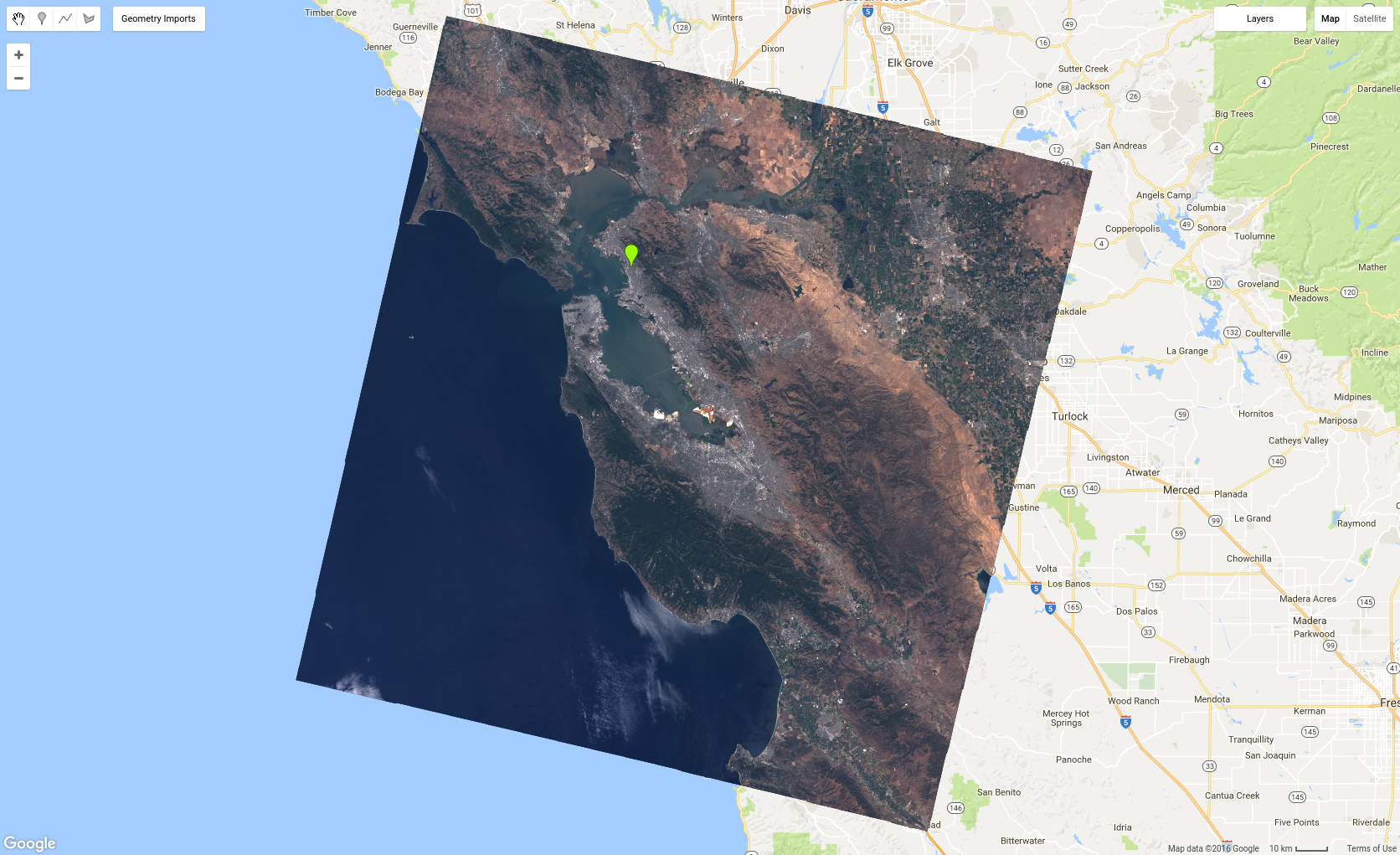
var visParams = {bands: ['B4', 'B3', 'B2'], max: 0.3};\nMap.addLayer(scene, visParams, 'true-color composite');\n```\n\nThe result should look something like Figure 5. Note that this code assigns the object\nof visualization parameters to a variable for possible future use. As you'll soon\ndiscover, that object will be useful when you visualize image collections!\nFigure 5. Landsat 8 TOA reflectance image as a true-color composite, stretched to \\[0, 0.3\\].\n\nTry playing with visualizing different bands. Another favorite combination is 'B5', 'B4',\nand 'B3' which is called a false-color composite. Some other interesting false-color\ncomposites are described\n[here](https://www.usgs.gov/media/images/common-landsat-band-rgb-composites).\n\nSince Earth Engine is designed to do large-scale analyses, you are not limited to working\nwith just one scene. Now it's time to display a whole collection as an RGB composite!\n\nDisplaying image collections\n----------------------------\n\nAdding an image collection to a map is similar to adding an image to a map. For\nexample, using 2016 images in the `l8` collection and the `visParams`\nobject defined previously,\n\n### Code Editor (JavaScript)\n\n```javascript\nvar l8 = ee.ImageCollection('LANDSAT/LC08/C02/T1_TOA');\nvar landsat2016 = l8.filterDate('2016-01-01', '2016-12-31');\nMap.addLayer(landsat2016, visParams, 'l8 collection');\n```\n\nNote that now you can zoom out and see a continuous mosaic where Landsat imagery\nis collected (i.e. over land). Also note that when you use the **Inspector**\ntab and click on the image, you'll see a list of pixel values (or a chart) in the\n**Pixels** section and a list of image objects in the **Objects**\nsection of the inspector.\n\nIf you zoomed out enough, you probably noticed some clouds in the mosaic. When\nyou add an `ImageCollection` to the map, it is displayed as a recent-value\ncomposite, meaning that only the most recent pixels are displayed (like calling\n`mosaic()` on the collection). That is why you can see discontinuities between\n[paths](http://landsat.gsfc.nasa.gov/?p=3231) which were acquired at\ndifferent times. It's also why many areas may appear cloudy. In the next page, learn how\nto change the way the images are composited to get rid of those pesky clouds! \n[arrow_backPrevious page](/earth-engine/tutorials/tutorial_api_03) [Next pagearrow_forward](/earth-engine/tutorials/tutorial_api_05)"]]