在 GitHub 上查看源代码
Earth Engine 中有多种光谱转换方法。这些方法包括针对图片的实例方法,例如 normalizedDifference()、unmix()、rgbToHsv() 和 hsvToRgb()。
平移锐化
通过分辨率更高的相应全色图像提供的增强功能,全景锐化可提高多波段图像的分辨率。
rgbToHsv() 和 hsvToRgb() 方法对平移锐化很有用。
Code Editor (JavaScript)
// Load a Landsat 8 top-of-atmosphere reflectance image.
var image = ee.Image('LANDSAT/LC08/C02/T1_TOA/LC08_044034_20140318');
Map.addLayer(
    image,
    {bands: ['B4', 'B3', 'B2'], min: 0, max: 0.25, gamma: [1.1, 1.1, 1]},
    'rgb');

// Convert the RGB bands to the HSV color space.
var hsv = image.select(['B4', 'B3', 'B2']).rgbToHsv();

// Swap in the panchromatic band and convert back to RGB.
var sharpened = ee.Image.cat([
  hsv.select('hue'), hsv.select('saturation'), image.select('B8')
]).hsvToRgb();

// Display the pan-sharpened result.
Map.setCenter(-122.44829, 37.76664, 13);
Map.addLayer(sharpened,
             {min: 0, max: 0.25, gamma: [1.3, 1.3, 1.3]},
             'pan-sharpened');
import ee
import geemap.core as geemap
Colab (Python)
# Load a Landsat 8 top-of-atmosphere reflectance image.
image = ee.Image('LANDSAT/LC08/C02/T1_TOA/LC08_044034_20140318')

# Convert the RGB bands to the HSV color space.
hsv = image.select(['B4', 'B3', 'B2']).rgbToHsv()

# Swap in the panchromatic band and convert back to RGB.
sharpened = ee.Image.cat(
    [hsv.select('hue'), hsv.select('saturation'), image.select('B8')]
).hsvToRgb()

# Define a map centered on San Francisco, California.
map_sharpened = geemap.Map(center=[37.76664, -122.44829], zoom=13)

# Add the image layers to the map and display it.
map_sharpened.add_layer(
    image,
    {
        'bands': ['B4', 'B3', 'B2'],
        'min': 0,
        'max': 0.25,
        'gamma': [1.1, 1.1, 1],
    },
    'rgb',
)
map_sharpened.add_layer(
    sharpened,
    {'min': 0, 'max': 0.25, 'gamma': [1.3, 1.3, 1.3]},
    'pan-sharpened',
)
display(map_sharpened)
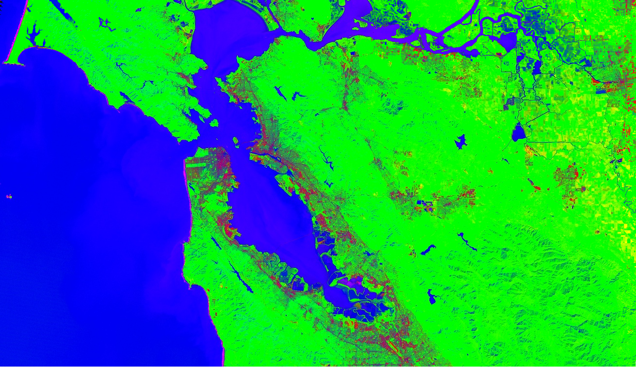
光谱分离
在 Earth Engine 中,光谱分解是作为 image.unmix() 方法实现的。
(如需了解更灵活的方法,请参阅“数组转换”页面)。以下是使用预先确定的城市、植被和水端元解混 Landsat 5 数据的示例:
Code Editor (JavaScript)
// Load a Landsat 5 image and select the bands we want to unmix.
var bands = ['B1', 'B2', 'B3', 'B4', 'B5', 'B6', 'B7'];
var image = ee.Image('LANDSAT/LT05/C02/T1/LT05_044034_20080214')
  .select(bands);
Map.setCenter(-122.1899, 37.5010, 10); // San Francisco Bay
Map.addLayer(image, {bands: ['B4', 'B3', 'B2'], min: 0, max: 128}, 'image');

// Define spectral endmembers.
var urban = [88, 42, 48, 38, 86, 115, 59];
var veg = [50, 21, 20, 35, 50, 110, 23];
var water = [51, 20, 14, 9, 7, 116, 4];

// Unmix the image.
var fractions = image.unmix([urban, veg, water]);
Map.addLayer(fractions, {}, 'unmixed');
import ee
import geemap.core as geemap
Colab (Python)
# Load a Landsat 5 image and select the bands we want to unmix.
bands = ['B1', 'B2', 'B3', 'B4', 'B5', 'B6', 'B7']
image = ee.Image('LANDSAT/LT05/C02/T1/LT05_044034_20080214').select(bands)

# Define spectral endmembers.
urban = [88, 42, 48, 38, 86, 115, 59]
veg = [50, 21, 20, 35, 50, 110, 23]
water = [51, 20, 14, 9, 7, 116, 4]

# Unmix the image.
fractions = image.unmix([urban, veg, water])

# Define a map centered on San Francisco Bay.
map_fractions = geemap.Map(center=[37.5010, -122.1899], zoom=10)

# Add the image layers to the map and display it.
map_fractions.add_layer(
    image, {'bands': ['B4', 'B3', 'B2'], 'min': 0, 'max': 128}, 'image'
)
map_fractions.add_layer(fractions, None, 'unmixed')
display(map_fractions)