我们先从创建波段所需的计算开始,该波段显示了 Hansen 等人提供的数据中既有损失又有增加的像素。
Hansen 等人的数据集包含一个像素值为 1(表示发生损失)或 0(表示未发生损失)的波段 (loss),以及一个像素值为 1(表示发生增益)或 0(表示未发生增益)的波段 (gain)。如需创建一个波段,其中 loss 和 gain 波段中的像素值均为 1,您可以使用图像的 and() 逻辑方法。and() 方法的调用方式为 image1.and(image2),并返回一个图像,其中 image1 和 image2 均为 1 的像素为 1,其他像素为 0:
代码编辑器 (JavaScript)
// Load the data and select the bands of interest.
var gfc2014 = ee.Image('UMD/hansen/global_forest_change_2015');
var lossImage = gfc2014.select(['loss']);
var gainImage = gfc2014.select(['gain']);

// Use the and() method to create the lossAndGain image.
var gainAndLoss = gainImage.and(lossImage);

// Show the loss and gain image.
Map.addLayer(gainAndLoss.updateMask(gainAndLoss),
    {palette: 'FF00FF'}, 'Gain and Loss');
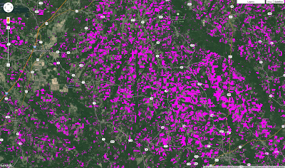
结果应如图 1 所示,其中显示了放大后的阿肯色州卫星视图。
将此示例与上一部分的结果相结合,现在可以重现本教程开头的图表:
代码编辑器 (JavaScript)
// Displaying forest, loss, gain, and pixels where both loss and gain occur.
var gfc2014 = ee.Image('UMD/hansen/global_forest_change_2015');
var lossImage = gfc2014.select(['loss']);
var gainImage = gfc2014.select(['gain']);
var treeCover = gfc2014.select(['treecover2000']);

// Use the and() method to create the lossAndGain image.
var gainAndLoss = gainImage.and(lossImage);

// Add the tree cover layer in green.
Map.addLayer(treeCover.updateMask(treeCover),
    {palette: ['000000', '00FF00'], max: 100}, 'Forest Cover');

// Add the loss layer in red.
Map.addLayer(lossImage.updateMask(lossImage),
    {palette: ['FF0000']}, 'Loss');

// Add the gain layer in blue.
Map.addLayer(gainImage.updateMask(gainImage),
    {palette: ['0000FF']}, 'Gain');

// Show the loss and gain image.
Map.addLayer(gainAndLoss.updateMask(gainAndLoss),
    {palette: 'FF00FF'}, 'Gain and Loss');
量化感兴趣区域的森林变化
现在,您已经比较熟悉 Hansen 等人数据集中的波段,接下来可以使用目前所学的概念来计算感兴趣区域的森林增加和减少统计信息。为此,我们需要使用矢量数据(点、线和多边形)。矢量数据集在 Earth Engine 中表示为 FeatureCollection。
(详细了解要素集合以及如何导入矢量数据。)
在本部分中,我们将比较刚果共和国在 2012 年发生的森林损失总量与该国保护区在同一时间发生的森林损失量。
正如您在 Earth Engine API 教程中所了解到的,用于计算图像区域统计信息的主要方法是 reduceRegion()。(详细了解如何减少图片区域。)例如,假设我们想计算研究期间估计的森林损失像素数。为此,请考虑以下代码:
代码编辑器 (JavaScript)
// Load country features from Large Scale International Boundary (LSIB) dataset.
var countries = ee.FeatureCollection('USDOS/LSIB_SIMPLE/2017');

// Subset the Congo Republic feature from countries.
var congo = countries.filter(ee.Filter.eq('country_na', 'Rep of the Congo'));

// Get the forest loss image.
var gfc2014 = ee.Image('UMD/hansen/global_forest_change_2015');
var lossImage = gfc2014.select(['loss']);

// Sum the values of forest loss pixels in the Congo Republic.
var stats = lossImage.reduceRegion({
  reducer: ee.Reducer.sum(),
  geometry: congo,
  scale: 30
});
print(stats);
此示例使用 ee.Reducer.sum() 归约器来对 congo 特征中 lossImage 内的像素值求和。由于 lossImage 由值为 1 或 0(分别表示丢失或未丢失)的像素组成,因此这些值的总和相当于区域中丢失的像素数。
遗憾的是,按原样运行脚本会导致如下错误:
reduceRegion() 中的默认最大像素数为 1,000 万。此错误消息表示刚果共和国覆盖了大约 3.83 亿个 Landsat 像素。幸运的是,reduceRegion() 接受许多参数,其中一个参数 (maxPixels) 可让您控制计算中使用的像素数。指定此参数可使计算成功完成:
代码编辑器 (JavaScript)
// Load country features from Large Scale International Boundary (LSIB) dataset.
var countries = ee.FeatureCollection('USDOS/LSIB_SIMPLE/2017');

// Subset the Congo Republic feature from countries.
var congo = countries.filter(ee.Filter.eq('country_na', 'Rep of the Congo'));

// Get the forest loss image.
var gfc2014 = ee.Image('UMD/hansen/global_forest_change_2015');
var lossImage = gfc2014.select(['loss']);

// Sum the values of forest loss pixels in the Congo Republic.
var stats = lossImage.reduceRegion({
  reducer: ee.Reducer.sum(),
  geometry: congo,
  scale: 30,
  maxPixels: 1e9
});
print(stats);
展开打印到控制台的对象,可以看到结果是损失了 4897933 像素的森林。您可以通过标记输出并从 reduceRegion() 返回的字典中获取感兴趣的结果,稍微清理一下控制台中的打印输出:
代码编辑器 (JavaScript)
print('pixels representing loss: ', stats.get('loss'));
计算像素面积
您很快就能回答以下问题:刚果共和国损失了多少面积的森林,其中有多少位于保护区内。剩余部分是将像素转换为实际面积。这种转换非常重要,因为我们不一定知道输入到 reduceRegion() 的像素大小。为了帮助计算面积,Earth Engine 提供了 ee.Image.pixelArea() 方法,该方法会生成一个图像,其中每个像素的值都是相应像素的面积(以平方米为单位)。将损失图像与此面积图像相乘,然后对结果求和,即可得到面积度量:
代码编辑器 (JavaScript)
// Load country features from Large Scale International Boundary (LSIB) dataset.
var countries = ee.FeatureCollection('USDOS/LSIB_SIMPLE/2017');

// Subset the Congo Republic feature from countries.
var congo = countries.filter(ee.Filter.eq('country_na', 'Rep of the Congo'));

// Get the forest loss image.
var gfc2014 = ee.Image('UMD/hansen/global_forest_change_2015');
var lossImage = gfc2014.select(['loss']);
var areaImage = lossImage.multiply(ee.Image.pixelArea());

// Sum the values of forest loss pixels in the Congo Republic.
var stats = areaImage.reduceRegion({
  reducer: ee.Reducer.sum(),
  geometry: congo,
  scale: 30,
  maxPixels: 1e9
});
print('pixels representing loss: ', stats.get('loss'), 'square meters');
现在,结果为研究期间损失了 4,372,575,052 平方米的森林。
现在,您已准备好回答本部分开头提出的问题:刚果共和国在 2012 年损失了多少森林面积,其中有多少位于保护区?
代码编辑器 (JavaScript)
// Load country features from Large Scale International Boundary (LSIB) dataset.
var countries = ee.FeatureCollection('USDOS/LSIB_SIMPLE/2017');

// Subset the Congo Republic feature from countries.
var congo = ee.Feature(
  countries
    .filter(ee.Filter.eq('country_na', 'Rep of the Congo'))
    .first()
);

// Subset protected areas to the bounds of the congo feature
// and other criteria. Clip to the intersection with congo.
var protectedAreas = ee.FeatureCollection('WCMC/WDPA/current/polygons')
  .filter(ee.Filter.and(
    ee.Filter.bounds(congo.geometry()),
    ee.Filter.neq('IUCN_CAT', 'VI'),
    ee.Filter.neq('STATUS', 'proposed'),
    ee.Filter.lt('STATUS_YR', 2010)
  ))
  .map(function(feat){
    return congo.intersection(feat);
  });

// Get the loss image.
var gfc2014 = ee.Image('UMD/hansen/global_forest_change_2015');
var lossIn2012 = gfc2014.select(['lossyear']).eq(12);
var areaImage = lossIn2012.multiply(ee.Image.pixelArea());

// Calculate the area of loss pixels in the Congo Republic.
var stats = areaImage.reduceRegion({
  reducer: ee.Reducer.sum(),
  geometry: congo.geometry(),
  scale: 30,
  maxPixels: 1e9
});
print(
  'Area lost in the Congo Republic:',
  stats.get('lossyear'),
  'square meters'
);

// Calculate the area of loss pixels in the protected areas.
var stats = areaImage.reduceRegion({
  reducer: ee.Reducer.sum(),
  geometry: protectedAreas.geometry(),
  scale: 30,
  maxPixels: 1e9
});
print(
  'Area lost in protected areas:',
  stats.get('lossyear'),
  'square meters'
);
输出结果表明,在 2012 年刚果共和国损失的 348,036,295 平方米森林中,有 11,880,976 平方米位于保护区内,如世界保护区数据库表所示。
此脚本与前一个脚本之间的唯一变化是添加了保护区信息,并将脚本从查看总体损失更改为查看 2012 年的损失。这需要进行两项更改。首先,有一个新的 lossIn2012 图像,其中 2012 年记录了损失的位置为 1,其他位置为 0。其次,由于频段的名称不同(lossyear 而不是 loss),因此必须在 print 语句中更改属性名称。
在下一部分中,我们将探索一些高级方法,用于计算和绘制每年的森林损失情况,而不是像本部分中那样只计算一年的森林损失情况。