선형 회귀

Earth Engine에는 리듀서를 사용하여 선형 회귀를 실행하는 여러 가지 방법이 있습니다.

• ee.Reducer.linearFit()
• ee.Reducer.linearRegression()
• ee.Reducer.robustLinearRegression()
• ee.Reducer.ridgeRegression()

가장 간단한 선형 회귀 감소 함수는 linearFit()로, 상수가 있는 단일 변수 선형 함수의 최소 제곱 추정치를 계산합니다. 선형 모델링에 더 유연한 접근 방식을 사용하려면 독립 변수와 종속 변수의 개수를 가변적으로 허용하는 선형 회귀 감소 도구 중 하나를 사용하세요. linearRegression()는 일반 최소 제곱 회귀(OLS)를 구현합니다. robustLinearRegression()는 회귀 잔차를 기반으로 하는 비용 함수를 사용하여 데이터에서 외부값의 가중치를 반복적으로 줄입니다(O’Leary, 1990). ridgeRegression()는 L2 정규화를 사용하여 선형 회귀를 실행합니다.

이러한 메서드를 사용한 회귀 분석은 ee.ImageCollection, ee.Image, ee.FeatureCollection, ee.List 객체를 줄이는 데 적합합니다. 다음 예는 각 항목의 애플리케이션을 보여줍니다. linearRegression(), robustLinearRegression(), ridgeRegression()는 모두 동일한 입력 및 출력 구조를 갖지만 linearFit()는 2밴드 입력 (X 뒤에 Y)을 예상하고 ridgeRegression()에는 추가 매개변수(lambda, 선택사항)와 출력 (pValue)이 있습니다.

참고: matrixSolve()는 ee.Reducer로 구현되지 않은 최소 제곱 회귀의 대체 메서드를 제공합니다.

ee.ImageCollection

linearFit()

데이터는 첫 번째 밴드가 독립 변수이고 두 번째 밴드가 종속 변수인 2밴드 입력 이미지로 설정해야 합니다. 다음 예는 기후 모델에 의해 예측된 향후 강수량의 선형 추세 (NEX-DCP30 데이터의 2006년 이후) 추정치를 보여줍니다. 종속 변수는 예상 강수량이고 독립 변수는 linearFit()를 호출하기 전에 추가된 시간입니다.

코드 편집기 (JavaScript)

// This function adds a time band to the image.
var createTimeBand = function(image) {
  // Scale milliseconds by a large constant to avoid very small slopes
  // in the linear regression output.
  return image.addBands(image.metadata('system:time_start').divide(1e18));
};

// Load the input image collection: projected climate data.
var collection = ee.ImageCollection('NASA/NEX-DCP30_ENSEMBLE_STATS')
  .filter(ee.Filter.eq('scenario', 'rcp85'))
  .filterDate(ee.Date('2006-01-01'), ee.Date('2050-01-01'))
  // Map the time band function over the collection.
  .map(createTimeBand);

// Reduce the collection with the linear fit reducer.
// Independent variable are followed by dependent variables.
var linearFit = collection.select(['system:time_start', 'pr_mean'])
  .reduce(ee.Reducer.linearFit());

// Display the results.
Map.setCenter(-100.11, 40.38, 5);
Map.addLayer(linearFit,
  {min: 0, max: [-0.9, 8e-5, 1], bands: ['scale', 'offset', 'scale']}, 'fit');

출력에는 '오프셋'(절편)과 '스케일'이라는 두 개의 대역이 포함됩니다. 이 맥락에서 '스케일'은 선의 기울기를 나타내며 많은 리듀서에 입력되는 스케일 매개변수(공간 스케일)와 혼동해서는 안 됩니다. 결과는 증가 추세가 있는 영역은 파란색, 감소 추세가 있는 영역은 빨간색, 추세가 없는 영역은 녹색으로 표시되며 그림 1과 같이 표시됩니다.

그림 1. 예측된 강수량에 적용된 linearFit()의 출력입니다. 강수량이 증가할 것으로 예상되는 지역은 파란색으로, 강수량이 감소할 것으로 예상되는 지역은 빨간색으로 표시됩니다.

linearRegression()

예를 들어 두 개의 종속 변수(강수량 및 최대 기온)와 두 개의 독립 변수(상수 및 시간)가 있다고 가정해 보겠습니다. 컬렉션은 이전 예와 동일하지만 감소하기 전에 상수 밴드를 수동으로 추가해야 합니다. 입력의 처음 두 밴드는 'X'(독립) 변수이고 다음 두 밴드는 'Y'(종속) 변수입니다. 이 예에서는 먼저 회귀 계수를 가져온 다음 배열 이미지를 평면화하여 관심 있는 밴드를 추출합니다.

코드 편집기 (JavaScript)

// This function adds a time band to the image.
var createTimeBand = function(image) {
  // Scale milliseconds by a large constant.
  return image.addBands(image.metadata('system:time_start').divide(1e18));
};

// This function adds a constant band to the image.
var createConstantBand = function(image) {
  return ee.Image(1).addBands(image);
};

// Load the input image collection: projected climate data.
var collection = ee.ImageCollection('NASA/NEX-DCP30_ENSEMBLE_STATS')
  .filterDate(ee.Date('2006-01-01'), ee.Date('2099-01-01'))
  .filter(ee.Filter.eq('scenario', 'rcp85'))
  // Map the functions over the collection, to get constant and time bands.
  .map(createTimeBand)
  .map(createConstantBand)
  // Select the predictors and the responses.
  .select(['constant', 'system:time_start', 'pr_mean', 'tasmax_mean']);

// Compute ordinary least squares regression coefficients.
var linearRegression = collection.reduce(
  ee.Reducer.linearRegression({
    numX: 2,
    numY: 2
}));

// Compute robust linear regression coefficients.
var robustLinearRegression = collection.reduce(
  ee.Reducer.robustLinearRegression({
    numX: 2,
    numY: 2
}));

// The results are array images that must be flattened for display.
// These lists label the information along each axis of the arrays.
var bandNames = [['constant', 'time'], // 0-axis variation.
                 ['precip', 'temp']]; // 1-axis variation.

// Flatten the array images to get multi-band images according to the labels.
var lrImage = linearRegression.select(['coefficients']).arrayFlatten(bandNames);
var rlrImage = robustLinearRegression.select(['coefficients']).arrayFlatten(bandNames);

// Display the OLS results.
Map.setCenter(-100.11, 40.38, 5);
Map.addLayer(lrImage,
  {min: 0, max: [-0.9, 8e-5, 1], bands: ['time_precip', 'constant_precip', 'time_precip']}, 'OLS');

// Compare the results at a specific point:
print('OLS estimates:', lrImage.reduceRegion({
  reducer: ee.Reducer.first(),
  geometry: ee.Geometry.Point([-96.0, 41.0]),
  scale: 1000
}));

print('Robust estimates:', rlrImage.reduceRegion({
  reducer: ee.Reducer.first(),
  geometry: ee.Geometry.Point([-96.0, 41.0]),
  scale: 1000
}));

결과를 검사하여 linearRegression() 출력이 linearFit() 감소기에 의해 추정된 계수와 동일한지 확인합니다. 단, linearRegression() 출력에는 다른 종속 변수인 tasmax_mean의 계수도 있습니다. 견고한 선형 회귀 계수는 OLS 추정치와 다릅니다. 이 예에서는 특정 지점에서 여러 회귀 방법의 계수를 비교합니다.

ee.Image

ee.Image 객체의 컨텍스트에서 회귀 감소기를 reduceRegion 또는 reduceRegions와 함께 사용하여 영역의 픽셀에 선형 회귀를 실행할 수 있습니다. 다음 예에서는 임의의 다각형에서 Landsat 밴드 간의 회귀 계수를 계산하는 방법을 보여줍니다.

linearFit()

배열 데이터 차트를 설명하는 가이드 섹션에는 Landsat 8 SWIR1 및 SWIR2 밴드 간의 상관관계에 관한 산점도가 표시됩니다. 여기에서 이 관계의 선형 회귀 계수가 계산됩니다. 'offset' (y 절편) 및 'scale' (기울기) 속성이 포함된 사전이 반환됩니다.

코드 편집기 (JavaScript)

// Define a rectangle geometry around San Francisco.
var sanFrancisco = ee.Geometry.Rectangle([-122.45, 37.74, -122.4, 37.8]);

// Import a Landsat 8 TOA image for this region.
var img = ee.Image('LANDSAT/LC08/C02/T1_TOA/LC08_044034_20140318');

// Subset the SWIR1 and SWIR2 bands. In the regression reducer, independent
// variables come first followed by the dependent variables. In this case,
// B5 (SWIR1) is the independent variable and B6 (SWIR2) is the dependent
// variable.
var imgRegress = img.select(['B5', 'B6']);

// Calculate regression coefficients for the set of pixels intersecting the
// above defined region using reduceRegion with ee.Reducer.linearFit().
var linearFit = imgRegress.reduceRegion({
  reducer: ee.Reducer.linearFit(),
  geometry: sanFrancisco,
  scale: 30,
});

// Inspect the results.
print('OLS estimates:', linearFit);
print('y-intercept:', linearFit.get('offset'));
print('Slope:', linearFit.get('scale'));

linearRegression()

이전 linearFit 섹션의 동일한 분석이 여기에 적용되지만 이번에는 ee.Reducer.linearRegression 함수가 사용됩니다. 회귀 이미지는 상수 이미지와 동일한 Landsat 8 이미지의 SWIR1 및 SWIR2 밴드를 나타내는 이미지 등 세 개의 개별 이미지로 구성됩니다. ee.Reducer.linearRegression를 사용하여 영역 감소를 위한 입력 이미지를 구성하기 위해 어떤 밴드 세트를 조합할 수도 있습니다. 밴드가 동일한 소스 이미지에 속할 필요는 없습니다.

코드 편집기 (JavaScript)

// Define a rectangle geometry around San Francisco.
var sanFrancisco = ee.Geometry.Rectangle([-122.45, 37.74, -122.4, 37.8]);

// Import a Landsat 8 TOA image for this region.
var img = ee.Image('LANDSAT/LC08/C02/T1_TOA/LC08_044034_20140318');

// Create a new image that is the concatenation of three images: a constant,
// the SWIR1 band, and the SWIR2 band.
var constant = ee.Image(1);
var xVar = img.select('B5');
var yVar = img.select('B6');
var imgRegress = ee.Image.cat(constant, xVar, yVar);

// Calculate regression coefficients for the set of pixels intersecting the
// above defined region using reduceRegion. The numX parameter is set as 2
// because the constant and the SWIR1 bands are independent variables and they
// are the first two bands in the stack; numY is set as 1 because there is only
// one dependent variable (SWIR2) and it follows as band three in the stack.
var linearRegression = imgRegress.reduceRegion({
  reducer: ee.Reducer.linearRegression({
    numX: 2,
    numY: 1
  }),
  geometry: sanFrancisco,
  scale: 30,
});

// Convert the coefficients array to a list.
var coefList = ee.Array(linearRegression.get('coefficients')).toList();

// Extract the y-intercept and slope.
var b0 = ee.List(coefList.get(0)).get(0); // y-intercept
var b1 = ee.List(coefList.get(1)).get(0); // slope

// Extract the residuals.
var residuals = ee.Array(linearRegression.get('residuals')).toList().get(0);

// Inspect the results.
print('OLS estimates', linearRegression);
print('y-intercept:', b0);
print('Slope:', b1);
print('Residuals:', residuals);

'coefficients' 및 'residuals' 속성이 포함된 사전이 반환됩니다. 'coefficients' 속성은 크기가 (numX, numY)인 배열입니다. 각 열에는 해당하는 종속 변수의 계수가 포함됩니다. 이 경우 배열에는 행 2개와 열 1개가 있습니다. 첫 번째 행의 첫 번째 열은 y절편이고 두 번째 행의 첫 번째 열은 기울기입니다. 'residuals' 속성은 각 종속 변수의 잔차의 제곱 평균 제곱근 벡터입니다. 결과를 배열로 변환한 다음 원하는 요소를 슬라이스하거나 배열을 목록으로 변환하고 색인 위치별로 계수를 선택하여 계수를 추출합니다.

ee.FeatureCollection

Sentinel-2와 Landsat 8 SWIR1 반사율 간의 선형 관계를 알고 싶다고 가정해 보겠습니다. 이 예에서는 점의 지형지물 컬렉션 형식의 무작위 픽셀 샘플이 관계를 계산하는 데 사용됩니다. 최적의 적합선인 최소 제곱 선과 함께 픽셀 쌍의 산점도가 생성됩니다 (그림 2).

코드 편집기 (JavaScript)

// Import a Sentinel-2 TOA image.
var s2ImgSwir1 = ee.Image('COPERNICUS/S2/20191022T185429_20191022T185427_T10SEH');

// Import a Landsat 8 TOA image from 12 days earlier than the S2 image.
var l8ImgSwir1 = ee.Image('LANDSAT/LC08/C02/T1_TOA/LC08_044033_20191010');

// Get the intersection between the two images - the area of interest (aoi).
var aoi = s2ImgSwir1.geometry().intersection(l8ImgSwir1.geometry());

// Get a set of 1000 random points from within the aoi. A feature collection
// is returned.
var sample = ee.FeatureCollection.randomPoints({
  region: aoi,
  points: 1000
});

// Combine the SWIR1 bands from each image into a single image.
var swir1Bands = s2ImgSwir1.select('B11')
  .addBands(l8ImgSwir1.select('B6'))
  .rename(['s2_swir1', 'l8_swir1']);

// Sample the SWIR1 bands using the sample point feature collection.
var imgSamp = swir1Bands.sampleRegions({
  collection: sample,
  scale: 30
})
// Add a constant property to each feature to be used as an independent variable.
.map(function(feature) {
  return feature.set('constant', 1);
});

// Compute linear regression coefficients. numX is 2 because
// there are two independent variables: 'constant' and 's2_swir1'. numY is 1
// because there is a single dependent variable: 'l8_swir1'. Cast the resulting
// object to an ee.Dictionary for easy access to the properties.
var linearRegression = ee.Dictionary(imgSamp.reduceColumns({
  reducer: ee.Reducer.linearRegression({
    numX: 2,
    numY: 1
  }),
  selectors: ['constant', 's2_swir1', 'l8_swir1']
}));

// Convert the coefficients array to a list.
var coefList = ee.Array(linearRegression.get('coefficients')).toList();

// Extract the y-intercept and slope.
var yInt = ee.List(coefList.get(0)).get(0); // y-intercept
var slope = ee.List(coefList.get(1)).get(0); // slope

// Gather the SWIR1 values from the point sample into a list of lists.
var props = ee.List(['s2_swir1', 'l8_swir1']);
var regressionVarsList = ee.List(imgSamp.reduceColumns({
  reducer: ee.Reducer.toList().repeat(props.size()),
  selectors: props
}).get('list'));

// Convert regression x and y variable lists to an array - used later as input
// to ui.Chart.array.values for generating a scatter plot.
var x = ee.Array(ee.List(regressionVarsList.get(0)));
var y1 = ee.Array(ee.List(regressionVarsList.get(1)));

// Apply the line function defined by the slope and y-intercept of the
// regression to the x variable list to create an array that will represent
// the regression line in the scatter plot.
var y2 = ee.Array(ee.List(regressionVarsList.get(0)).map(function(x) {
  var y = ee.Number(x).multiply(slope).add(yInt);
  return y;
}));

// Concatenate the y variables (Landsat 8 SWIR1 and predicted y) into an array
// for input to ui.Chart.array.values for plotting a scatter plot.
var yArr = ee.Array.cat([y1, y2], 1);

// Make a scatter plot of the two SWIR1 bands for the point sample and include
// the least squares line of best fit through the data.
print(ui.Chart.array.values({
  array: yArr,
  axis: 0,
  xLabels: x})
  .setChartType('ScatterChart')
  .setOptions({
    legend: {position: 'none'},
    hAxis: {'title': 'Sentinel-2 SWIR1'},
    vAxis: {'title': 'Landsat 8 SWIR1'},
    series: {
      0: {
        pointSize: 0.2,
        dataOpacity: 0.5,
      },
      1: {
        pointSize: 0,
        lineWidth: 2,
      }
    }
  })
);

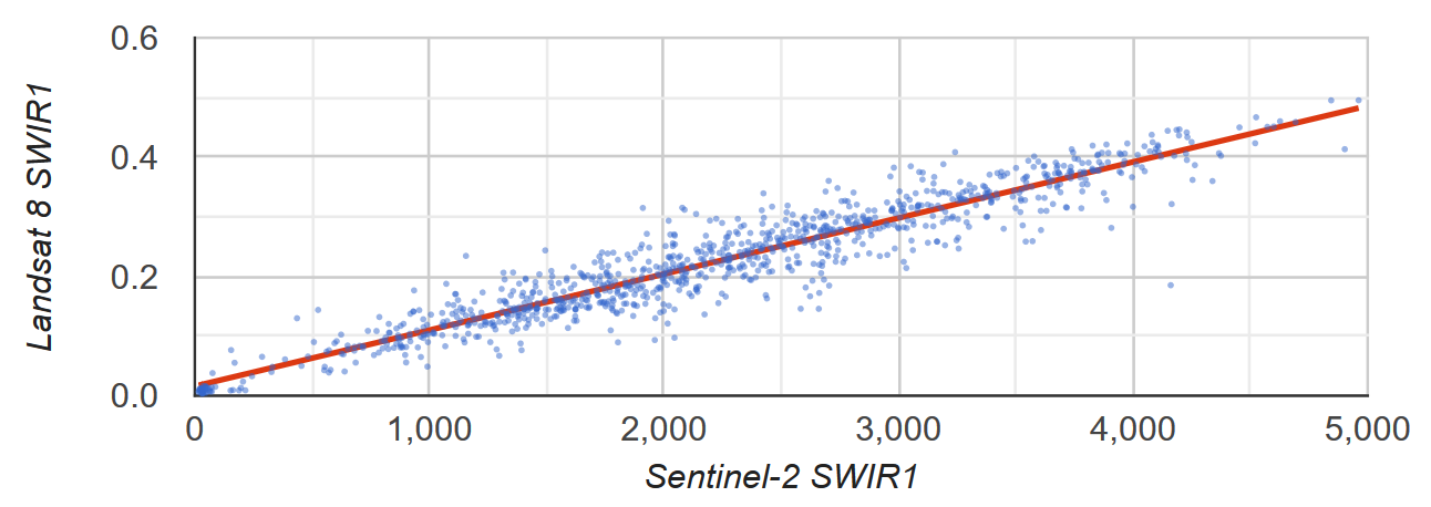
그림 2 Sentinel-2 및 Landsat 8 SWIR1 TOA 반사율을 나타내는 샘플 픽셀의 산점도 및 최소 제곱 선형 회귀 선

ee.List

2D ee.List 객체의 열은 회귀 감소기에 입력될 수 있습니다. 다음 예는 간단한 증명을 제공합니다. 독립 변수는 y 절편이 0이고 기울기가 1인 종속 변수의 사본입니다.

참고: ee.List 감소의 결과는 객체입니다. 속성에 더 쉽게 액세스할 수 있도록 ee.Dictionary로 변환합니다.

주의: 행과 열의 길이는 같아야 합니다. 누락된 데이터 항목을 나타내려면 null를 사용하세요.

linearFit()

코드 편집기 (JavaScript)

// Define a list of lists, where columns represent variables. The first column
// is the independent variable and the second is the dependent variable.
var listsVarColumns = ee.List([
  [1, 1],
  [2, 2],
  [3, 3],
  [4, 4],
  [5, 5]
]);

// Compute the least squares estimate of a linear function. Note that an
// object is returned; cast it as an ee.Dictionary to make accessing the
// coefficients easier.
var linearFit = ee.Dictionary(listsVarColumns.reduce(ee.Reducer.linearFit()));

// Inspect the result.
print(linearFit);
print('y-intercept:', linearFit.get('offset'));
print('Slope:', linearFit.get('scale'));

ee.Array로 변환하고 전치한 다음 다시 ee.List로 변환하여 변수가 행으로 표시되는 경우 목록을 전치합니다.

코드 편집기 (JavaScript)

// If variables in the list are arranged as rows, you'll need to transpose it.
// Define a list of lists where rows represent variables. The first row is the
// independent variable and the second is the dependent variable.
var listsVarRows = ee.List([
  [1, 2, 3, 4, 5],
  [1, 2, 3, 4, 5]
]);

// Cast the ee.List as an ee.Array, transpose it, and cast back to ee.List.
var listsVarColumns = ee.Array(listsVarRows).transpose().toList();

// Compute the least squares estimate of a linear function. Note that an
// object is returned; cast it as an ee.Dictionary to make accessing the
// coefficients easier.
var linearFit = ee.Dictionary(listsVarColumns.reduce(ee.Reducer.linearFit()));

// Inspect the result.
print(linearFit);
print('y-intercept:', linearFit.get('offset'));
print('Slope:', linearFit.get('scale'));

linearRegression()

ee.Reducer.linearRegression() 적용은 상수 독립 변수가 포함된다는 점을 제외하고 위의 linearFit() 예와 유사합니다.

코드 편집기 (JavaScript)

// Define a list of lists where columns represent variables. The first column
// represents a constant term, the second an independent variable, and the third
// a dependent variable.
var listsVarColumns = ee.List([
  [1, 1, 1],
  [1, 2, 2],
  [1, 3, 3],
  [1, 4, 4],
  [1, 5, 5]
]);

// Compute ordinary least squares regression coefficients. numX is 2 because
// there is one constant term and an additional independent variable. numY is 1
// because there is only a single dependent variable. Cast the resulting
// object to an ee.Dictionary for easy access to the properties.
var linearRegression = ee.Dictionary(
  listsVarColumns.reduce(ee.Reducer.linearRegression({
    numX: 2,
    numY: 1
})));

// Convert the coefficients array to a list.
var coefList = ee.Array(linearRegression.get('coefficients')).toList();

// Extract the y-intercept and slope.
var b0 = ee.List(coefList.get(0)).get(0); // y-intercept
var b1 = ee.List(coefList.get(1)).get(0); // slope

// Extract the residuals.
var residuals = ee.Array(linearRegression.get('residuals')).toList().get(0);

// Inspect the results.
print('OLS estimates', linearRegression);
print('y-intercept:', b0);
print('Slope:', b1);
print('Residuals:', residuals);