Regresja liniowa

Earth Engine ma kilka metod wykonywania regresji liniowej za pomocą reduktora:

• ee.Reducer.linearFit()
• ee.Reducer.linearRegression()
• ee.Reducer.robustLinearRegression()
• ee.Reducer.ridgeRegression()

Najprostszym reduktorem regresji liniowej jest linearFit(), który oblicza szacunek metodą najmniejszych kwadratów funkcji liniowej jednej zmiennej z wykładnikiem stałym. Aby zastosować bardziej elastyczne podejście do modelowania liniowego, użyj jednego z reduktorów regresji liniowej, który umożliwia zmienną liczbę zmiennych niezależnych i zależnych. linearRegression() stosuje regresję metodą najmniejszych kwadratów(OLS). robustLinearRegression() używa funkcji kosztu opartej na resztach regresji, aby stopniowo zmniejszać wagę wartości odstających w danych (O’Leary, 1990). Funkcja ridgeRegression() wykonuje regresję liniową z regularyzacją L2.

Analiza regresji z użyciem tych metod jest odpowiednia do zmniejszania liczby obiektów ee.ImageCollection, ee.Image, ee.FeatureCollection i ee.List. Poniższe przykłady pokazują, jak można ich używać. Pamiętaj, że funkcje linearRegression(), robustLinearRegression() i ridgeRegression() mają te same struktury wejścia i wyjścia, ale funkcja linearFit() oczekuje dwupasmowego wejścia (X, a następnie Y), a funkcja ridgeRegression() ma dodatkowy parametr (lambda, opcjonalny) i wyjście (pValue).

Uwaga: matrixSolve() pozwala na zastosowanie alternatywnej metody regresji najmniejszych kwadratów, która nie jest implementowana jako ee.Reducer.

ee.ImageCollection

linearFit()

Dane powinny być skonfigurowane jako obraz wejściowy o 2 pasmach, gdzie pierwszy pas jest zmienną niezależną, a drugi – zmienną zależną. Poniższy przykład pokazuje oszacowanie trendu liniowego przyszłych opadów (po 2006 r. w danych NEX-DCP30) prognozowane przez modele klimatyczne. Zmienną zależną jest prognozowany poziom opadów, a zmienną niezależną jest czas, dodany przed wywołaniem funkcji linearFit():

Edytor kodu (JavaScript)

// This function adds a time band to the image.
var createTimeBand = function(image) {
  // Scale milliseconds by a large constant to avoid very small slopes
  // in the linear regression output.
  return image.addBands(image.metadata('system:time_start').divide(1e18));
};

// Load the input image collection: projected climate data.
var collection = ee.ImageCollection('NASA/NEX-DCP30_ENSEMBLE_STATS')
  .filter(ee.Filter.eq('scenario', 'rcp85'))
  .filterDate(ee.Date('2006-01-01'), ee.Date('2050-01-01'))
  // Map the time band function over the collection.
  .map(createTimeBand);

// Reduce the collection with the linear fit reducer.
// Independent variable are followed by dependent variables.
var linearFit = collection.select(['system:time_start', 'pr_mean'])
  .reduce(ee.Reducer.linearFit());

// Display the results.
Map.setCenter(-100.11, 40.38, 5);
Map.addLayer(linearFit,
  {min: 0, max: [-0.9, 8e-5, 1], bands: ['scale', 'offset', 'scale']}, 'fit');

Zauważ, że dane wyjściowe zawierają 2 pasma: „offset” (punkt przecięcia) i „skala” („skala” w tym kontekście odnosi się do nachylenia linii i nie należy go mylić z parametrem skali podawanym jako dane wejściowe wielu reduktorom, który jest skalą przestrzenną). Wynik, czyli obszary trendu wzrostowego w kolorze niebieskim, trendu spadkowego w kolorze czerwonym i brak trendu w kolorze zielonym, powinien wyglądać mniej więcej tak jak na rysunku 1.

Rysunek 1. Wynik funkcji linearFit() zastosowany do prognozowanych opadów. Obszary, na których prognozowane są zwiększone opady, są zaznaczone na niebiesko, a obszary z mniejszymi opadami – na czerwono.

linearRegression()

Załóżmy np., że istnieją 2 zmiennej zależne: opady i maksymalna temperatura oraz 2 zmiennych niezależnych: stała i czas. Kolekcja jest identyczna jak w poprzednim przykładzie, ale pasmo stałe musi zostać dodane ręcznie przed zmniejszeniem. Pierwsze 2 pasma wejścia to zmienne „X” (niezależne), a kolejne 2 pasma to zmienne „Y” (zależne). W tym przykładzie najpierw uzyskaj współczynniki regresji, a potem spłaszcz obraz tablicy, aby wyodrębnić interesujące pasma:

Edytor kodu (JavaScript)

// This function adds a time band to the image.
var createTimeBand = function(image) {
  // Scale milliseconds by a large constant.
  return image.addBands(image.metadata('system:time_start').divide(1e18));
};

// This function adds a constant band to the image.
var createConstantBand = function(image) {
  return ee.Image(1).addBands(image);
};

// Load the input image collection: projected climate data.
var collection = ee.ImageCollection('NASA/NEX-DCP30_ENSEMBLE_STATS')
  .filterDate(ee.Date('2006-01-01'), ee.Date('2099-01-01'))
  .filter(ee.Filter.eq('scenario', 'rcp85'))
  // Map the functions over the collection, to get constant and time bands.
  .map(createTimeBand)
  .map(createConstantBand)
  // Select the predictors and the responses.
  .select(['constant', 'system:time_start', 'pr_mean', 'tasmax_mean']);

// Compute ordinary least squares regression coefficients.
var linearRegression = collection.reduce(
  ee.Reducer.linearRegression({
    numX: 2,
    numY: 2
}));

// Compute robust linear regression coefficients.
var robustLinearRegression = collection.reduce(
  ee.Reducer.robustLinearRegression({
    numX: 2,
    numY: 2
}));

// The results are array images that must be flattened for display.
// These lists label the information along each axis of the arrays.
var bandNames = [['constant', 'time'], // 0-axis variation.
                 ['precip', 'temp']]; // 1-axis variation.

// Flatten the array images to get multi-band images according to the labels.
var lrImage = linearRegression.select(['coefficients']).arrayFlatten(bandNames);
var rlrImage = robustLinearRegression.select(['coefficients']).arrayFlatten(bandNames);

// Display the OLS results.
Map.setCenter(-100.11, 40.38, 5);
Map.addLayer(lrImage,
  {min: 0, max: [-0.9, 8e-5, 1], bands: ['time_precip', 'constant_precip', 'time_precip']}, 'OLS');

// Compare the results at a specific point:
print('OLS estimates:', lrImage.reduceRegion({
  reducer: ee.Reducer.first(),
  geometry: ee.Geometry.Point([-96.0, 41.0]),
  scale: 1000
}));

print('Robust estimates:', rlrImage.reduceRegion({
  reducer: ee.Reducer.first(),
  geometry: ee.Geometry.Point([-96.0, 41.0]),
  scale: 1000
}));

Po sprawdzeniu wyników możesz zauważyć, że dane wyjściowe linearRegression() są równoważne współczynnikom oszacowanym przez reduktor linearFit(), ale dane wyjściowe linearRegression() zawierają też współczynniki dla innej zmiennej zależnej, tasmax_mean. Współczynniki robust regresji liniowej różnią się od oszacowań OLS. W tym przykładzie porównano współczynniki różnych metod regresji w określonym punkcie.

ee.Image

W kontekście obiektu ee.Image można używać reduktora regresji z funkcją reduceRegion lub reduceRegions, aby wykonać regresję liniową na pikselach w regionie lub regionach. W poniższych przykładach pokazano, jak obliczyć współczynniki regresji między pasmami Landsat w dowolnym wielokącie.

linearFit()

W sekcji przewodnika poświęconej diagramom danych tablicowych znajdziesz wykres punktowy korelacji między pasmami SWIR1 i SWIR2 obrazu Landsat 8. Tutaj obliczane są współczynniki regresji liniowej dla tego związku. Zwracany jest słownik zawierający właściwości 'offset' (punkt przecięcia z osią Y) i 'scale' (nachylenie).

Edytor kodu (JavaScript)

// Define a rectangle geometry around San Francisco.
var sanFrancisco = ee.Geometry.Rectangle([-122.45, 37.74, -122.4, 37.8]);

// Import a Landsat 8 TOA image for this region.
var img = ee.Image('LANDSAT/LC08/C02/T1_TOA/LC08_044034_20140318');

// Subset the SWIR1 and SWIR2 bands. In the regression reducer, independent
// variables come first followed by the dependent variables. In this case,
// B5 (SWIR1) is the independent variable and B6 (SWIR2) is the dependent
// variable.
var imgRegress = img.select(['B5', 'B6']);

// Calculate regression coefficients for the set of pixels intersecting the
// above defined region using reduceRegion with ee.Reducer.linearFit().
var linearFit = imgRegress.reduceRegion({
  reducer: ee.Reducer.linearFit(),
  geometry: sanFrancisco,
  scale: 30,
});

// Inspect the results.
print('OLS estimates:', linearFit);
print('y-intercept:', linearFit.get('offset'));
print('Slope:', linearFit.get('scale'));

linearRegression()

Tutaj stosujemy tę samą analizę co w poprzedniej sekcji linearFit, z tą różnicą, że tym razem używamy funkcji ee.Reducer.linearRegression. Pamiętaj, że obraz regresji jest tworzony z 3 osobnych obrazów: obrazu stałego oraz obrazów reprezentujących pasma SWIR1 i SWIR2 z tego samego obrazu Landsat 8. Pamiętaj, że możesz połączyć dowolny zestaw pasm, aby utworzyć obraz wejściowy do redukcji regionu za pomocą funkcji ee.Reducer.linearRegression. Nie muszą one należeć do tego samego obrazu źródłowego.

Edytor kodu (JavaScript)

// Define a rectangle geometry around San Francisco.
var sanFrancisco = ee.Geometry.Rectangle([-122.45, 37.74, -122.4, 37.8]);

// Import a Landsat 8 TOA image for this region.
var img = ee.Image('LANDSAT/LC08/C02/T1_TOA/LC08_044034_20140318');

// Create a new image that is the concatenation of three images: a constant,
// the SWIR1 band, and the SWIR2 band.
var constant = ee.Image(1);
var xVar = img.select('B5');
var yVar = img.select('B6');
var imgRegress = ee.Image.cat(constant, xVar, yVar);

// Calculate regression coefficients for the set of pixels intersecting the
// above defined region using reduceRegion. The numX parameter is set as 2
// because the constant and the SWIR1 bands are independent variables and they
// are the first two bands in the stack; numY is set as 1 because there is only
// one dependent variable (SWIR2) and it follows as band three in the stack.
var linearRegression = imgRegress.reduceRegion({
  reducer: ee.Reducer.linearRegression({
    numX: 2,
    numY: 1
  }),
  geometry: sanFrancisco,
  scale: 30,
});

// Convert the coefficients array to a list.
var coefList = ee.Array(linearRegression.get('coefficients')).toList();

// Extract the y-intercept and slope.
var b0 = ee.List(coefList.get(0)).get(0); // y-intercept
var b1 = ee.List(coefList.get(1)).get(0); // slope

// Extract the residuals.
var residuals = ee.Array(linearRegression.get('residuals')).toList().get(0);

// Inspect the results.
print('OLS estimates', linearRegression);
print('y-intercept:', b0);
print('Slope:', b1);
print('Residuals:', residuals);

Zwracany jest słownik zawierający właściwości 'coefficients' i 'residuals'. Właściwość 'coefficients' to tablica o wymiarach (numX, numY); każda kolumna zawiera współczynniki odpowiadającej zmiennej zależnej. W tym przypadku tablica ma 2 wiersze i 1 kolumnę:wiersz 1, kolumna 1 to odcięta na osi y, a wiersz 2, kolumna 1 to nachylenie. Właściwość 'residuals' to wektor średniej kwadratowej wartości pozostałości dla każdej zmiennej zależnej. Wyodrębnij współczynniki, zmieniając wynik w tablicę, a następnie wyodrębniając z niej odpowiednie elementy. Możesz też przekształcić tablicę w listę i wybrać współczynniki według pozycji indeksu.

ee.FeatureCollection

Załóżmy, że chcesz poznać zależność liniową między Sentinel-2 a odblaskiem SWIR1 Landsat 8. W tym przykładzie do obliczenia relacji użyto losowej próbki pikseli sformatowanych jako zbiór cech punktów. Generowany jest wykres punktowy par pikseli wraz z linią trendu najmniejszych kwadratów (ryc. 2).

Edytor kodu (JavaScript)

// Import a Sentinel-2 TOA image.
var s2ImgSwir1 = ee.Image('COPERNICUS/S2/20191022T185429_20191022T185427_T10SEH');

// Import a Landsat 8 TOA image from 12 days earlier than the S2 image.
var l8ImgSwir1 = ee.Image('LANDSAT/LC08/C02/T1_TOA/LC08_044033_20191010');

// Get the intersection between the two images - the area of interest (aoi).
var aoi = s2ImgSwir1.geometry().intersection(l8ImgSwir1.geometry());

// Get a set of 1000 random points from within the aoi. A feature collection
// is returned.
var sample = ee.FeatureCollection.randomPoints({
  region: aoi,
  points: 1000
});

// Combine the SWIR1 bands from each image into a single image.
var swir1Bands = s2ImgSwir1.select('B11')
  .addBands(l8ImgSwir1.select('B6'))
  .rename(['s2_swir1', 'l8_swir1']);

// Sample the SWIR1 bands using the sample point feature collection.
var imgSamp = swir1Bands.sampleRegions({
  collection: sample,
  scale: 30
})
// Add a constant property to each feature to be used as an independent variable.
.map(function(feature) {
  return feature.set('constant', 1);
});

// Compute linear regression coefficients. numX is 2 because
// there are two independent variables: 'constant' and 's2_swir1'. numY is 1
// because there is a single dependent variable: 'l8_swir1'. Cast the resulting
// object to an ee.Dictionary for easy access to the properties.
var linearRegression = ee.Dictionary(imgSamp.reduceColumns({
  reducer: ee.Reducer.linearRegression({
    numX: 2,
    numY: 1
  }),
  selectors: ['constant', 's2_swir1', 'l8_swir1']
}));

// Convert the coefficients array to a list.
var coefList = ee.Array(linearRegression.get('coefficients')).toList();

// Extract the y-intercept and slope.
var yInt = ee.List(coefList.get(0)).get(0); // y-intercept
var slope = ee.List(coefList.get(1)).get(0); // slope

// Gather the SWIR1 values from the point sample into a list of lists.
var props = ee.List(['s2_swir1', 'l8_swir1']);
var regressionVarsList = ee.List(imgSamp.reduceColumns({
  reducer: ee.Reducer.toList().repeat(props.size()),
  selectors: props
}).get('list'));

// Convert regression x and y variable lists to an array - used later as input
// to ui.Chart.array.values for generating a scatter plot.
var x = ee.Array(ee.List(regressionVarsList.get(0)));
var y1 = ee.Array(ee.List(regressionVarsList.get(1)));

// Apply the line function defined by the slope and y-intercept of the
// regression to the x variable list to create an array that will represent
// the regression line in the scatter plot.
var y2 = ee.Array(ee.List(regressionVarsList.get(0)).map(function(x) {
  var y = ee.Number(x).multiply(slope).add(yInt);
  return y;
}));

// Concatenate the y variables (Landsat 8 SWIR1 and predicted y) into an array
// for input to ui.Chart.array.values for plotting a scatter plot.
var yArr = ee.Array.cat([y1, y2], 1);

// Make a scatter plot of the two SWIR1 bands for the point sample and include
// the least squares line of best fit through the data.
print(ui.Chart.array.values({
  array: yArr,
  axis: 0,
  xLabels: x})
  .setChartType('ScatterChart')
  .setOptions({
    legend: {position: 'none'},
    hAxis: {'title': 'Sentinel-2 SWIR1'},
    vAxis: {'title': 'Landsat 8 SWIR1'},
    series: {
      0: {
        pointSize: 0.2,
        dataOpacity: 0.5,
      },
      1: {
        pointSize: 0,
        lineWidth: 2,
      }
    }
  })
);

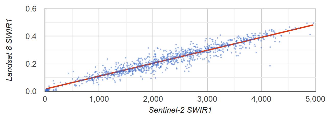
Rysunek 2. Wykres rozrzutu i linia regresji liniowej najmniejszych kwadratów dla próbki pikseli reprezentujących odbicie TOA SWIR1 Sentinel-2 i Landsat 8.

ee.List

Kolumny obiektów dwuwymiarowych ee.List mogą być wejściami funkcji regresji. Poniżej znajdziesz proste dowody. Zmienne niezależne to kopie zmiennych zależnych, które dają punkt przecięcia osi y równy 0 i nachylenie równe 1.

Uwaga: wynik działania ee.List jest obiektem. Przekształć go w ee.Dictionary, aby ułatwić dostęp do właściwości.

Uwaga: długości wierszy i kolumn muszą być równe. Użyj wartości null, aby reprezentować brakujące wpisy danych.

linearFit()

Edytor kodu (JavaScript)

// Define a list of lists, where columns represent variables. The first column
// is the independent variable and the second is the dependent variable.
var listsVarColumns = ee.List([
  [1, 1],
  [2, 2],
  [3, 3],
  [4, 4],
  [5, 5]
]);

// Compute the least squares estimate of a linear function. Note that an
// object is returned; cast it as an ee.Dictionary to make accessing the
// coefficients easier.
var linearFit = ee.Dictionary(listsVarColumns.reduce(ee.Reducer.linearFit()));

// Inspect the result.
print(linearFit);
print('y-intercept:', linearFit.get('offset'));
print('Slope:', linearFit.get('scale'));

Jeśli zmienne są reprezentowane przez wiersze, przetransponuj listę, przekształcając ją w macierz ee.Array, a potem przekształcając ją z powrotem w macierz ee.List.

Edytor kodu (JavaScript)

// If variables in the list are arranged as rows, you'll need to transpose it.
// Define a list of lists where rows represent variables. The first row is the
// independent variable and the second is the dependent variable.
var listsVarRows = ee.List([
  [1, 2, 3, 4, 5],
  [1, 2, 3, 4, 5]
]);

// Cast the ee.List as an ee.Array, transpose it, and cast back to ee.List.
var listsVarColumns = ee.Array(listsVarRows).transpose().toList();

// Compute the least squares estimate of a linear function. Note that an
// object is returned; cast it as an ee.Dictionary to make accessing the
// coefficients easier.
var linearFit = ee.Dictionary(listsVarColumns.reduce(ee.Reducer.linearFit()));

// Inspect the result.
print(linearFit);
print('y-intercept:', linearFit.get('offset'));
print('Slope:', linearFit.get('scale'));

linearRegression()

Zastosowanie funkcji ee.Reducer.linearRegression() jest podobne do przykładu funkcji linearFit(), z tą różnicą, że uwzględnia ona stałą zmienną niezależną.

Edytor kodu (JavaScript)

// Define a list of lists where columns represent variables. The first column
// represents a constant term, the second an independent variable, and the third
// a dependent variable.
var listsVarColumns = ee.List([
  [1, 1, 1],
  [1, 2, 2],
  [1, 3, 3],
  [1, 4, 4],
  [1, 5, 5]
]);

// Compute ordinary least squares regression coefficients. numX is 2 because
// there is one constant term and an additional independent variable. numY is 1
// because there is only a single dependent variable. Cast the resulting
// object to an ee.Dictionary for easy access to the properties.
var linearRegression = ee.Dictionary(
  listsVarColumns.reduce(ee.Reducer.linearRegression({
    numX: 2,
    numY: 1
})));

// Convert the coefficients array to a list.
var coefList = ee.Array(linearRegression.get('coefficients')).toList();

// Extract the y-intercept and slope.
var b0 = ee.List(coefList.get(0)).get(0); // y-intercept
var b1 = ee.List(coefList.get(1)).get(0); // slope

// Extract the residuals.
var residuals = ee.Array(linearRegression.get('residuals')).toList().get(0);

// Inspect the results.
print('OLS estimates', linearRegression);
print('y-intercept:', b0);
print('Slope:', b1);
print('Residuals:', residuals);