Regressão linear

O Earth Engine tem vários métodos para realizar regressões lineares usando redutores:

• ee.Reducer.linearFit()
• ee.Reducer.linearRegression()
• ee.Reducer.robustLinearRegression()
• ee.Reducer.ridgeRegression()

O redutor de regressão linear mais simples é linearFit(), que calcula a estimativa de mínimos quadrados de uma função linear de uma variável com um termo constante. Para uma abordagem mais flexível da modelagem linear, use um dos redutores de regressão linear que permitem um número variável de variáveis independentes e dependentes. linearRegression() implementa a regressão dos mínimos quadrados ordinários(OLS). robustLinearRegression() usa uma função de custo baseada em resíduos de regressão para reduzir de forma iterativa os valores atípicos nos dados (O’Leary, 1990). ridgeRegression() faz uma regressão linear com regularização L2.

A análise de regressão com esses métodos é adequada para reduzir os objetos ee.ImageCollection, ee.Image, ee.FeatureCollection e ee.List. Os exemplos a seguir demonstram uma aplicação para cada um. linearRegression(), robustLinearRegression() e ridgeRegression() têm as mesmas estruturas de entrada e saída, mas linearFit() espera uma entrada de duas bandas (X seguida de Y) e ridgeRegression() tem um parâmetro adicional (lambda, opcional) e saída (pValue).

Observação: matrixSolve() oferece um método alternativo para a regressão linear simples que não é implementado como um ee.Reducer.

ee.ImageCollection

linearFit()

Os dados precisam ser configurados como uma imagem de entrada de duas bandas, em que a primeira banda é a variável independente e a segunda é a variável dependente. O exemplo a seguir mostra a estimativa da tendência linear de precipitação futura (após 2006 nos dados NEX-DCP30) projetada por modelos climáticos. A variável dependente é a precipitação projetada, e a variável independente é o tempo, adicionado antes de chamar linearFit():

Editor de código (JavaScript)

// This function adds a time band to the image.
var createTimeBand = function(image) {
  // Scale milliseconds by a large constant to avoid very small slopes
  // in the linear regression output.
  return image.addBands(image.metadata('system:time_start').divide(1e18));
};

// Load the input image collection: projected climate data.
var collection = ee.ImageCollection('NASA/NEX-DCP30_ENSEMBLE_STATS')
  .filter(ee.Filter.eq('scenario', 'rcp85'))
  .filterDate(ee.Date('2006-01-01'), ee.Date('2050-01-01'))
  // Map the time band function over the collection.
  .map(createTimeBand);

// Reduce the collection with the linear fit reducer.
// Independent variable are followed by dependent variables.
var linearFit = collection.select(['system:time_start', 'pr_mean'])
  .reduce(ee.Reducer.linearFit());

// Display the results.
Map.setCenter(-100.11, 40.38, 5);
Map.addLayer(linearFit,
  {min: 0, max: [-0.9, 8e-5, 1], bands: ['scale', 'offset', 'scale']}, 'fit');

Observe que a saída contém duas faixas, o "offset" (interceptação) e a "escala" (neste contexto, "escala" se refere à inclinação da linha e não deve ser confundida com a entrada do parâmetro de escala de muitos redutores, que é a escala espacial). O resultado, com áreas de tendência crescente em azul, tendência decrescente em vermelho e nenhuma tendência em verde, deve ser semelhante à Figura 1.

Figura 1. A saída de linearFit() aplicada à precipitação prevista. As áreas com previsão de aumento de precipitação são mostradas em azul, e as com diminuição, em vermelho.

linearRegression()

Por exemplo, suponha que haja duas variáveis dependentes: precipitação e temperatura máxima, e duas variáveis independentes: uma constante e o tempo. A coleção é idêntica ao exemplo anterior, mas a faixa constante precisa ser adicionada manualmente antes da redução. As duas primeiras faixas da entrada são as variáveis "X" (independentes) e as duas próximas são as variáveis "Y" (dependentes). Neste exemplo, primeiro extraia os coeficientes de regressão e depois abra a imagem da matriz para extrair as faixas de interesse:

Editor de código (JavaScript)

// This function adds a time band to the image.
var createTimeBand = function(image) {
  // Scale milliseconds by a large constant.
  return image.addBands(image.metadata('system:time_start').divide(1e18));
};

// This function adds a constant band to the image.
var createConstantBand = function(image) {
  return ee.Image(1).addBands(image);
};

// Load the input image collection: projected climate data.
var collection = ee.ImageCollection('NASA/NEX-DCP30_ENSEMBLE_STATS')
  .filterDate(ee.Date('2006-01-01'), ee.Date('2099-01-01'))
  .filter(ee.Filter.eq('scenario', 'rcp85'))
  // Map the functions over the collection, to get constant and time bands.
  .map(createTimeBand)
  .map(createConstantBand)
  // Select the predictors and the responses.
  .select(['constant', 'system:time_start', 'pr_mean', 'tasmax_mean']);

// Compute ordinary least squares regression coefficients.
var linearRegression = collection.reduce(
  ee.Reducer.linearRegression({
    numX: 2,
    numY: 2
}));

// Compute robust linear regression coefficients.
var robustLinearRegression = collection.reduce(
  ee.Reducer.robustLinearRegression({
    numX: 2,
    numY: 2
}));

// The results are array images that must be flattened for display.
// These lists label the information along each axis of the arrays.
var bandNames = [['constant', 'time'], // 0-axis variation.
                 ['precip', 'temp']]; // 1-axis variation.

// Flatten the array images to get multi-band images according to the labels.
var lrImage = linearRegression.select(['coefficients']).arrayFlatten(bandNames);
var rlrImage = robustLinearRegression.select(['coefficients']).arrayFlatten(bandNames);

// Display the OLS results.
Map.setCenter(-100.11, 40.38, 5);
Map.addLayer(lrImage,
  {min: 0, max: [-0.9, 8e-5, 1], bands: ['time_precip', 'constant_precip', 'time_precip']}, 'OLS');

// Compare the results at a specific point:
print('OLS estimates:', lrImage.reduceRegion({
  reducer: ee.Reducer.first(),
  geometry: ee.Geometry.Point([-96.0, 41.0]),
  scale: 1000
}));

print('Robust estimates:', rlrImage.reduceRegion({
  reducer: ee.Reducer.first(),
  geometry: ee.Geometry.Point([-96.0, 41.0]),
  scale: 1000
}));

Inspecione os resultados para descobrir que a saída linearRegression() é equivalente aos coeficientes estimados pelo redutor linearFit(), embora a saída linearRegression() também tenha coeficientes para a outra variável dependente, tasmax_mean. Os coeficientes de regressão linear robustos são diferentes das estimativas de OLS. O exemplo compara os coeficientes dos diferentes métodos de regressão em um ponto específico.

ee.Image

No contexto de um objeto ee.Image, os redutores de regressão podem ser usados com reduceRegion ou reduceRegions para realizar uma regressão linear nos pixels das regiões. Os exemplos a seguir demonstram como calcular coeficientes de regressão entre as bandas do Landsat em um polígono arbitrário.

linearFit()

A seção do guia que descreve os gráficos de dados de matriz mostra um diagrama de dispersão da correlação entre as bandas SWIR1 e SWIR2 do Landsat 8. Aqui, os coeficientes de regressão linear para essa relação são calculados. Um dicionário contendo as propriedades 'offset' (interseção do eixo y) e 'scale' (inclinação) é retornado.

Editor de código (JavaScript)

// Define a rectangle geometry around San Francisco.
var sanFrancisco = ee.Geometry.Rectangle([-122.45, 37.74, -122.4, 37.8]);

// Import a Landsat 8 TOA image for this region.
var img = ee.Image('LANDSAT/LC08/C02/T1_TOA/LC08_044034_20140318');

// Subset the SWIR1 and SWIR2 bands. In the regression reducer, independent
// variables come first followed by the dependent variables. In this case,
// B5 (SWIR1) is the independent variable and B6 (SWIR2) is the dependent
// variable.
var imgRegress = img.select(['B5', 'B6']);

// Calculate regression coefficients for the set of pixels intersecting the
// above defined region using reduceRegion with ee.Reducer.linearFit().
var linearFit = imgRegress.reduceRegion({
  reducer: ee.Reducer.linearFit(),
  geometry: sanFrancisco,
  scale: 30,
});

// Inspect the results.
print('OLS estimates:', linearFit);
print('y-intercept:', linearFit.get('offset'));
print('Slope:', linearFit.get('scale'));

linearRegression()

A mesma análise da seção linearFit anterior é aplicada aqui, exceto que desta vez a função ee.Reducer.linearRegression é usada. Uma imagem de regressão é construída a partir de três imagens separadas: uma imagem constante e imagens que representam as bandas SWIR1 e SWIR2 da mesma imagem do Landsat 8. É possível combinar qualquer conjunto de bandas para criar uma imagem de entrada para a redução de região por ee.Reducer.linearRegression. Elas não precisam pertencer à mesma imagem de origem.

Editor de código (JavaScript)

// Define a rectangle geometry around San Francisco.
var sanFrancisco = ee.Geometry.Rectangle([-122.45, 37.74, -122.4, 37.8]);

// Import a Landsat 8 TOA image for this region.
var img = ee.Image('LANDSAT/LC08/C02/T1_TOA/LC08_044034_20140318');

// Create a new image that is the concatenation of three images: a constant,
// the SWIR1 band, and the SWIR2 band.
var constant = ee.Image(1);
var xVar = img.select('B5');
var yVar = img.select('B6');
var imgRegress = ee.Image.cat(constant, xVar, yVar);

// Calculate regression coefficients for the set of pixels intersecting the
// above defined region using reduceRegion. The numX parameter is set as 2
// because the constant and the SWIR1 bands are independent variables and they
// are the first two bands in the stack; numY is set as 1 because there is only
// one dependent variable (SWIR2) and it follows as band three in the stack.
var linearRegression = imgRegress.reduceRegion({
  reducer: ee.Reducer.linearRegression({
    numX: 2,
    numY: 1
  }),
  geometry: sanFrancisco,
  scale: 30,
});

// Convert the coefficients array to a list.
var coefList = ee.Array(linearRegression.get('coefficients')).toList();

// Extract the y-intercept and slope.
var b0 = ee.List(coefList.get(0)).get(0); // y-intercept
var b1 = ee.List(coefList.get(1)).get(0); // slope

// Extract the residuals.
var residuals = ee.Array(linearRegression.get('residuals')).toList().get(0);

// Inspect the results.
print('OLS estimates', linearRegression);
print('y-intercept:', b0);
print('Slope:', b1);
print('Residuals:', residuals);

Um dicionário contendo as propriedades 'coefficients' e 'residuals' é retornado. A propriedade 'coefficients' é uma matriz com dimensões (numX, numY); cada coluna contém os coeficientes da variável dependente correspondente. Nesse caso, a matriz tem duas linhas e uma coluna: a primeira linha, a primeira coluna é a interseção em y, e a segunda linha, a primeira coluna é a inclinação. A propriedade 'residuals' é o vetor da raiz quadrada média dos resíduos de cada variável dependente. Extraia os coeficientes convertendo o resultado em uma matriz e, em seguida, cortando os elementos desejados ou convertendo a matriz em uma lista e selecionando os coeficientes por posição do índice.

ee.FeatureCollection

Suponha que você queira saber a relação linear entre o Sentinel-2 e a refletância SWIR1 do Landsat 8. Neste exemplo, uma amostra aleatória de pixels formatada como uma coleção de recursos de pontos é usada para calcular a relação. Um gráfico de dispersão dos pares de pixels com a linha de mínimos quadrados de melhor ajuste é gerado (Figura 2).

Editor de código (JavaScript)

// Import a Sentinel-2 TOA image.
var s2ImgSwir1 = ee.Image('COPERNICUS/S2/20191022T185429_20191022T185427_T10SEH');

// Import a Landsat 8 TOA image from 12 days earlier than the S2 image.
var l8ImgSwir1 = ee.Image('LANDSAT/LC08/C02/T1_TOA/LC08_044033_20191010');

// Get the intersection between the two images - the area of interest (aoi).
var aoi = s2ImgSwir1.geometry().intersection(l8ImgSwir1.geometry());

// Get a set of 1000 random points from within the aoi. A feature collection
// is returned.
var sample = ee.FeatureCollection.randomPoints({
  region: aoi,
  points: 1000
});

// Combine the SWIR1 bands from each image into a single image.
var swir1Bands = s2ImgSwir1.select('B11')
  .addBands(l8ImgSwir1.select('B6'))
  .rename(['s2_swir1', 'l8_swir1']);

// Sample the SWIR1 bands using the sample point feature collection.
var imgSamp = swir1Bands.sampleRegions({
  collection: sample,
  scale: 30
})
// Add a constant property to each feature to be used as an independent variable.
.map(function(feature) {
  return feature.set('constant', 1);
});

// Compute linear regression coefficients. numX is 2 because
// there are two independent variables: 'constant' and 's2_swir1'. numY is 1
// because there is a single dependent variable: 'l8_swir1'. Cast the resulting
// object to an ee.Dictionary for easy access to the properties.
var linearRegression = ee.Dictionary(imgSamp.reduceColumns({
  reducer: ee.Reducer.linearRegression({
    numX: 2,
    numY: 1
  }),
  selectors: ['constant', 's2_swir1', 'l8_swir1']
}));

// Convert the coefficients array to a list.
var coefList = ee.Array(linearRegression.get('coefficients')).toList();

// Extract the y-intercept and slope.
var yInt = ee.List(coefList.get(0)).get(0); // y-intercept
var slope = ee.List(coefList.get(1)).get(0); // slope

// Gather the SWIR1 values from the point sample into a list of lists.
var props = ee.List(['s2_swir1', 'l8_swir1']);
var regressionVarsList = ee.List(imgSamp.reduceColumns({
  reducer: ee.Reducer.toList().repeat(props.size()),
  selectors: props
}).get('list'));

// Convert regression x and y variable lists to an array - used later as input
// to ui.Chart.array.values for generating a scatter plot.
var x = ee.Array(ee.List(regressionVarsList.get(0)));
var y1 = ee.Array(ee.List(regressionVarsList.get(1)));

// Apply the line function defined by the slope and y-intercept of the
// regression to the x variable list to create an array that will represent
// the regression line in the scatter plot.
var y2 = ee.Array(ee.List(regressionVarsList.get(0)).map(function(x) {
  var y = ee.Number(x).multiply(slope).add(yInt);
  return y;
}));

// Concatenate the y variables (Landsat 8 SWIR1 and predicted y) into an array
// for input to ui.Chart.array.values for plotting a scatter plot.
var yArr = ee.Array.cat([y1, y2], 1);

// Make a scatter plot of the two SWIR1 bands for the point sample and include
// the least squares line of best fit through the data.
print(ui.Chart.array.values({
  array: yArr,
  axis: 0,
  xLabels: x})
  .setChartType('ScatterChart')
  .setOptions({
    legend: {position: 'none'},
    hAxis: {'title': 'Sentinel-2 SWIR1'},
    vAxis: {'title': 'Landsat 8 SWIR1'},
    series: {
      0: {
        pointSize: 0.2,
        dataOpacity: 0.5,
      },
      1: {
        pointSize: 0,
        lineWidth: 2,
      }
    }
  })
);

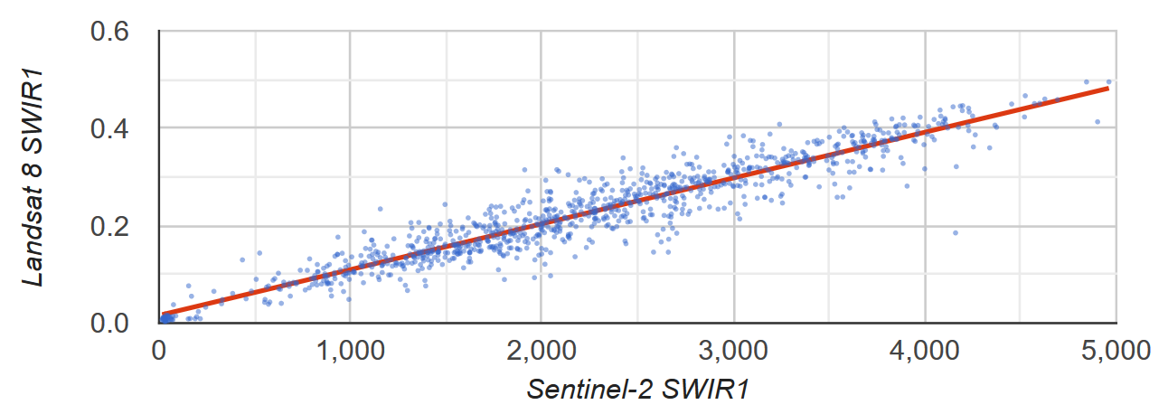
Figura 2. Diagrama de dispersão e linha de regressão linear dos quadrados mínimos para uma amostra de pixels que representam a refletância TOA SWIR1 do Sentinel-2 e do Landsat 8.

ee.List

As colunas de objetos ee.List bidimensionais podem ser entradas para redutores de regressão. Os exemplos a seguir fornecem provas simples. A variável independente é uma cópia da variável dependente que produz um valor de y igual a 0 e uma inclinação igual a 1.

Observação: o resultado da redução de ee.List é um objeto. Converta-o em um ee.Dictionary para facilitar o acesso às propriedades.

Cuidado: os comprimentos entre linhas e colunas precisam ser iguais. Use null para representar entradas de dados ausentes.

linearFit()

Editor de código (JavaScript)

// Define a list of lists, where columns represent variables. The first column
// is the independent variable and the second is the dependent variable.
var listsVarColumns = ee.List([
  [1, 1],
  [2, 2],
  [3, 3],
  [4, 4],
  [5, 5]
]);

// Compute the least squares estimate of a linear function. Note that an
// object is returned; cast it as an ee.Dictionary to make accessing the
// coefficients easier.
var linearFit = ee.Dictionary(listsVarColumns.reduce(ee.Reducer.linearFit()));

// Inspect the result.
print(linearFit);
print('y-intercept:', linearFit.get('offset'));
print('Slope:', linearFit.get('scale'));

Transponha a lista se as variáveis forem representadas por linhas convertendo-as em ee.Array, transpondo-as e convertendo-as de volta em ee.List.

Editor de código (JavaScript)

// If variables in the list are arranged as rows, you'll need to transpose it.
// Define a list of lists where rows represent variables. The first row is the
// independent variable and the second is the dependent variable.
var listsVarRows = ee.List([
  [1, 2, 3, 4, 5],
  [1, 2, 3, 4, 5]
]);

// Cast the ee.List as an ee.Array, transpose it, and cast back to ee.List.
var listsVarColumns = ee.Array(listsVarRows).transpose().toList();

// Compute the least squares estimate of a linear function. Note that an
// object is returned; cast it as an ee.Dictionary to make accessing the
// coefficients easier.
var linearFit = ee.Dictionary(listsVarColumns.reduce(ee.Reducer.linearFit()));

// Inspect the result.
print(linearFit);
print('y-intercept:', linearFit.get('offset'));
print('Slope:', linearFit.get('scale'));

linearRegression()

A aplicação de ee.Reducer.linearRegression() é semelhante ao exemplo linearFit() acima, exceto que uma variável independente constante é incluída.

Editor de código (JavaScript)

// Define a list of lists where columns represent variables. The first column
// represents a constant term, the second an independent variable, and the third
// a dependent variable.
var listsVarColumns = ee.List([
  [1, 1, 1],
  [1, 2, 2],
  [1, 3, 3],
  [1, 4, 4],
  [1, 5, 5]
]);

// Compute ordinary least squares regression coefficients. numX is 2 because
// there is one constant term and an additional independent variable. numY is 1
// because there is only a single dependent variable. Cast the resulting
// object to an ee.Dictionary for easy access to the properties.
var linearRegression = ee.Dictionary(
  listsVarColumns.reduce(ee.Reducer.linearRegression({
    numX: 2,
    numY: 1
})));

// Convert the coefficients array to a list.
var coefList = ee.Array(linearRegression.get('coefficients')).toList();

// Extract the y-intercept and slope.
var b0 = ee.List(coefList.get(0)).get(0); // y-intercept
var b1 = ee.List(coefList.get(1)).get(0); // slope

// Extract the residuals.
var residuals = ee.Array(linearRegression.get('residuals')).toList().get(0);

// Inspect the results.
print('OLS estimates', linearRegression);
print('y-intercept:', b0);
print('Slope:', b1);
print('Residuals:', residuals);