ประกาศ: โปรเจ็กต์ที่ไม่ใช่เชิงพาณิชย์ทั้งหมดที่ลงทะเบียนเพื่อใช้ Earth Engine ก่อนวันที่ 15 เมษายน 2025 ต้องยืนยันการมีสิทธิ์ที่ไม่ใช่เชิงพาณิชย์เพื่อรักษาสิทธิ์เข้าถึง Earth Engine

หน้านี้ได้รับการแปลโดย Cloud Translation API

การถดถอยเชิงเส้น

Earth Engine มีวิธีการหลายวิธีในการทำการถดถอยเชิงเส้นโดยใช้ตัวลด

ee.Reducer.linearFit()
ee.Reducer.linearRegression()
ee.Reducer.robustLinearRegression()
ee.Reducer.ridgeRegression()

ตัวลดขนาดการถดถอยเชิงเส้นที่ง่ายที่สุดคือ linearFit() ซึ่งจะคํานวณค่าประมาณกำลังสองน้อยที่สุดของฟังก์ชันเชิงเส้นของตัวแปรเดียวที่มีเทอมของค่าคงที่ หากต้องการใช้วิธีการประมาณเชิงเส้นที่ยืดหยุ่นมากขึ้น ให้ใช้ตัวลดการถดถอยเชิงเส้นอย่างใดอย่างหนึ่งที่อนุญาตให้มีตัวแปรอิสระและตัวแปรตามจํานวนเท่าใดก็ได้ linearRegression() ใช้การถดถอยแบบกำลังสองน้อยที่สุดแบบธรรมดา(OLS) robustLinearRegression() ใช้ฟังก์ชันต้นทุนที่อิงตามค่าคงเหลือของการถดถอยเพื่อลดน้ำหนักค่าผิดปกติในข้อมูลซ้ำๆ (O’Leary, 1990) ridgeRegression() ทําการถดถอยเชิงเส้นด้วย Regularization แบบ L2

การวิเคราะห์การถดถอยด้วยวิธีการเหล่านี้เหมาะสำหรับการลดออบเจ็กต์ ee.ImageCollection, ee.Image, ee.FeatureCollection และ ee.List ตัวอย่างต่อไปนี้แสดงการใช้งานของแต่ละรายการ โปรดทราบว่า linearRegression(), robustLinearRegression() และ ridgeRegression() ทั้งหมดมีโครงสร้างอินพุตและเอาต์พุตเหมือนกัน แต่ linearFit() ต้องการอินพุตแบบ 2 แบนด์ (X ตามด้วย Y) และ ridgeRegression() มีพารามิเตอร์เพิ่มเติม (lambda ซึ่งไม่บังคับ) และเอาต์พุต (pValue)

ee.ImageCollection

`linearFit()`

ควรตั้งค่าข้อมูลเป็นภาพอินพุต 2 ย่าน โดยย่านแรกคือตัวแปรอิสระ และย่านที่สองคือตัวแปรตาม ตัวอย่างต่อไปนี้แสดงค่าประมาณแนวโน้มเชิงเส้นของปริมาณน้ำฝนในอนาคต (หลังปี 2006 ในข้อมูล NEX-DCP30) ที่คาดการณ์โดยโมเดลสภาพอากาศ ตัวแปรตามคือปริมาณน้ำฝนที่คาดการณ์ และตัวแปรอิสระคือเวลา ซึ่งเพิ่มไว้ก่อนเรียกใช้ linearFit()

เครื่องมือแก้ไขโค้ด (JavaScript)

// This function adds a time band to the image.
var createTimeBand = function(image) {
  // Scale milliseconds by a large constant to avoid very small slopes
  // in the linear regression output.
  return image.addBands(image.metadata('system:time_start').divide(1e18));
};

// Load the input image collection: projected climate data.
var collection = ee.ImageCollection('NASA/NEX-DCP30_ENSEMBLE_STATS')
  .filter(ee.Filter.eq('scenario', 'rcp85'))
  .filterDate(ee.Date('2006-01-01'), ee.Date('2050-01-01'))
  // Map the time band function over the collection.
  .map(createTimeBand);

// Reduce the collection with the linear fit reducer.
// Independent variable are followed by dependent variables.
var linearFit = collection.select(['system:time_start', 'pr_mean'])
  .reduce(ee.Reducer.linearFit());

// Display the results.
Map.setCenter(-100.11, 40.38, 5);
Map.addLayer(linearFit,
  {min: 0, max: [-0.9, 8e-5, 1], bands: ['scale', 'offset', 'scale']}, 'fit');

โปรดทราบว่าเอาต์พุตมี 2 แถบ ได้แก่ "ค่าออฟเซต" (จุดตัด) และ "มาตราส่วน" ("มาตราส่วน" ในบริบทนี้หมายถึงความลาดชันของเส้นและไม่ควรสับสนกับอินพุตพารามิเตอร์มาตราส่วนที่ส่งไปยังตัวลดจํานวนหลายตัว ซึ่งเป็นมาตราส่วนเชิงพื้นที่) ผลลัพธ์ที่ได้จะมีลักษณะดังรูปที่ 1 ซึ่งแสดงพื้นที่ที่มีแนวโน้มเพิ่มขึ้นเป็นสีน้ำเงิน แนวโน้มลดลงเป็นสีแดง และไม่มีแนวโน้มเป็นสีเขียว

รูปที่ 1 เอาต์พุตของ linearFit() ใช้กับปริมาณน้ำฝนที่คาดการณ์ พื้นที่ที่คาดว่าจะมีปริมาณน้ำฝนเพิ่มขึ้นจะแสดงเป็นสีน้ำเงิน และพื้นที่ที่คาดว่าจะมีปริมาณน้ำฝนลดลงจะแสดงเป็นสีแดง

`linearRegression()`

เช่น สมมติว่าตัวแปรตามมี 2 รายการ ได้แก่ ปริมาณน้ำฝนและอุณหภูมิสูงสุด และตัวแปรอิสระมี 2 รายการ ได้แก่ ค่าคงที่และเวลา คอลเล็กชันนี้เหมือนกับตัวอย่างก่อนหน้า แต่ต้องเพิ่มแถบคงที่ด้วยตนเองก่อนการลด แถบ 2 แถวแรกของอินพุตคือตัวแปร "X" (อิสระ) และ 2 แถวถัดไปคือตัวแปร "Y" (ตาม) ในตัวอย่างนี้ ให้รับค่าสัมประสิทธิ์การถดถอยก่อน จากนั้นจึงผสานรูปภาพอาร์เรย์เพื่อดึงข้อมูลย่านความถี่ที่ต้องการ

เครื่องมือแก้ไขโค้ด (JavaScript)

// This function adds a time band to the image.
var createTimeBand = function(image) {
  // Scale milliseconds by a large constant.
  return image.addBands(image.metadata('system:time_start').divide(1e18));
};

// This function adds a constant band to the image.
var createConstantBand = function(image) {
  return ee.Image(1).addBands(image);
};

// Load the input image collection: projected climate data.
var collection = ee.ImageCollection('NASA/NEX-DCP30_ENSEMBLE_STATS')
  .filterDate(ee.Date('2006-01-01'), ee.Date('2099-01-01'))
  .filter(ee.Filter.eq('scenario', 'rcp85'))
  // Map the functions over the collection, to get constant and time bands.
  .map(createTimeBand)
  .map(createConstantBand)
  // Select the predictors and the responses.
  .select(['constant', 'system:time_start', 'pr_mean', 'tasmax_mean']);

// Compute ordinary least squares regression coefficients.
var linearRegression = collection.reduce(
  ee.Reducer.linearRegression({
    numX: 2,
    numY: 2
}));

// Compute robust linear regression coefficients.
var robustLinearRegression = collection.reduce(
  ee.Reducer.robustLinearRegression({
    numX: 2,
    numY: 2
}));

// The results are array images that must be flattened for display.
// These lists label the information along each axis of the arrays.
var bandNames = [['constant', 'time'], // 0-axis variation.
                 ['precip', 'temp']]; // 1-axis variation.

// Flatten the array images to get multi-band images according to the labels.
var lrImage = linearRegression.select(['coefficients']).arrayFlatten(bandNames);
var rlrImage = robustLinearRegression.select(['coefficients']).arrayFlatten(bandNames);

// Display the OLS results.
Map.setCenter(-100.11, 40.38, 5);
Map.addLayer(lrImage,
  {min: 0, max: [-0.9, 8e-5, 1], bands: ['time_precip', 'constant_precip', 'time_precip']}, 'OLS');

// Compare the results at a specific point:
print('OLS estimates:', lrImage.reduceRegion({
  reducer: ee.Reducer.first(),
  geometry: ee.Geometry.Point([-96.0, 41.0]),
  scale: 1000
}));

print('Robust estimates:', rlrImage.reduceRegion({
  reducer: ee.Reducer.first(),
  geometry: ee.Geometry.Point([-96.0, 41.0]),
  scale: 1000
}));

ตรวจสอบผลลัพธ์เพื่อดูว่าเอาต์พุต linearRegression() เทียบเท่ากับค่าสัมประสิทธิ์ที่ประมาณโดยตัวลด linearFit() แม้ว่าเอาต์พุต linearRegression() จะมีค่าสัมประสิทธิ์สำหรับตัวแปรตามอื่นๆ อย่าง tasmax_mean ด้วย สัมประสิทธิ์การถดถอยเชิงเส้นที่มีประสิทธิภาพจะแตกต่างจากค่าประมาณ OLS ตัวอย่างนี้เปรียบเทียบค่าสัมประสิทธิ์จากวิธีการหาค่าสัมพัทธ์ที่แตกต่างกัน ณ จุดหนึ่งๆ

ee.Image

ในบริบทของออบเจ็กต์ ee.Image คุณสามารถใช้ตัวลดการถดถอยร่วมกับ reduceRegion หรือ reduceRegions เพื่อทำการถดถอยเชิงเส้นกับพิกเซลในภูมิภาค ตัวอย่างต่อไปนี้แสดงวิธีคำนวณค่าสัมประสิทธิ์การถดถอยระหว่างย่านความถี่ของ Landsat ในรูปหลายเหลี่ยมที่กำหนดเอง

`linearFit()`

ส่วนคำแนะนำที่อธิบายแผนภูมิข้อมูลอาร์เรย์จะแสดงผังกระจายของความสัมพันธ์ระหว่างย่าน SWIR1 และ SWIR2 ของ Landsat 8 ระบบจะคํานวณค่าสัมประสิทธิ์การถดถอยเชิงเส้นสําหรับความสัมพันธ์นี้ ระบบจะแสดงพจนานุกรมที่มีพร็อพเพอร์ตี้ 'offset' (ค่าคงที่ y) และ 'scale' (ความชัน)

เครื่องมือแก้ไขโค้ด (JavaScript)

// Define a rectangle geometry around San Francisco.
var sanFrancisco = ee.Geometry.Rectangle([-122.45, 37.74, -122.4, 37.8]);

// Import a Landsat 8 TOA image for this region.
var img = ee.Image('LANDSAT/LC08/C02/T1_TOA/LC08_044034_20140318');

// Subset the SWIR1 and SWIR2 bands. In the regression reducer, independent
// variables come first followed by the dependent variables. In this case,
// B5 (SWIR1) is the independent variable and B6 (SWIR2) is the dependent
// variable.
var imgRegress = img.select(['B5', 'B6']);

// Calculate regression coefficients for the set of pixels intersecting the
// above defined region using reduceRegion with ee.Reducer.linearFit().
var linearFit = imgRegress.reduceRegion({
  reducer: ee.Reducer.linearFit(),
  geometry: sanFrancisco,
  scale: 30,
});

// Inspect the results.
print('OLS estimates:', linearFit);
print('y-intercept:', linearFit.get('offset'));
print('Slope:', linearFit.get('scale'));

`linearRegression()`

การวิเคราะห์เดียวกันจากส่วน linearFit ก่อนหน้านี้จะมีผลที่นี่ ยกเว้นครั้งนี้จะใช้ฟังก์ชัน ee.Reducer.linearRegression โปรดทราบว่ารูปภาพการถดถอยสร้างขึ้นจากรูปภาพ 3 รูปแยกกัน ได้แก่ รูปภาพคงที่และรูปภาพที่แสดงแถบ SWIR1 และ SWIR2 จากรูปภาพ Landsat 8 เดียวกัน โปรดทราบว่าคุณสามารถรวมชุดแถบใดก็ได้เพื่อสร้างรูปภาพอินพุตสำหรับการลดภูมิภาคตาม ee.Reducer.linearRegression โดยไม่จำเป็นต้องเป็นแถบจากรูปภาพต้นทางเดียวกัน

เครื่องมือแก้ไขโค้ด (JavaScript)

// Define a rectangle geometry around San Francisco.
var sanFrancisco = ee.Geometry.Rectangle([-122.45, 37.74, -122.4, 37.8]);

// Import a Landsat 8 TOA image for this region.
var img = ee.Image('LANDSAT/LC08/C02/T1_TOA/LC08_044034_20140318');

// Create a new image that is the concatenation of three images: a constant,
// the SWIR1 band, and the SWIR2 band.
var constant = ee.Image(1);
var xVar = img.select('B5');
var yVar = img.select('B6');
var imgRegress = ee.Image.cat(constant, xVar, yVar);

// Calculate regression coefficients for the set of pixels intersecting the
// above defined region using reduceRegion. The numX parameter is set as 2
// because the constant and the SWIR1 bands are independent variables and they
// are the first two bands in the stack; numY is set as 1 because there is only
// one dependent variable (SWIR2) and it follows as band three in the stack.
var linearRegression = imgRegress.reduceRegion({
  reducer: ee.Reducer.linearRegression({
    numX: 2,
    numY: 1
  }),
  geometry: sanFrancisco,
  scale: 30,
});

// Convert the coefficients array to a list.
var coefList = ee.Array(linearRegression.get('coefficients')).toList();

// Extract the y-intercept and slope.
var b0 = ee.List(coefList.get(0)).get(0); // y-intercept
var b1 = ee.List(coefList.get(1)).get(0); // slope

// Extract the residuals.
var residuals = ee.Array(linearRegression.get('residuals')).toList().get(0);

// Inspect the results.
print('OLS estimates', linearRegression);
print('y-intercept:', b0);
print('Slope:', b1);
print('Residuals:', residuals);

ระบบจะแสดงพจนานุกรมที่มีพร็อพเพอร์ตี้ 'coefficients' และ 'residuals' พร็อพเพอร์ตี้ 'coefficients' คืออาร์เรย์ที่มีมิติข้อมูล (numX, numY) แต่ละคอลัมน์มีสัมประสิทธิ์ของตัวแปรตามที่เกี่ยวข้อง ในกรณีนี้ อาร์เรย์มี 2 แถวและ 1 คอลัมน์ โดยแถวที่ 1 คอลัมน์ที่ 1 คือจุดตัด y และแถวที่ 2 คอลัมน์ที่ 1 คือความชัน พร็อพเพอร์ตี้ 'residuals' คือเวกเตอร์ของค่าเฉลี่ยกำลังสองของส่วนที่เหลือของตัวแปรตามแต่ละตัว ดึงค่าสัมประสิทธิ์โดยแคสต์ผลลัพธ์เป็นอาร์เรย์ แล้วตัดองค์ประกอบที่ต้องการออก หรือแปลงอาร์เรย์เป็นลิสต์แล้วเลือกค่าสัมประสิทธิ์ตามตำแหน่งดัชนี

ee.FeatureCollection

สมมติว่าคุณต้องการทราบความสัมพันธ์เชิงเส้นระหว่างการสะท้อนแสง SWIR1 ของ Sentinel-2 กับ Landsat 8 ในตัวอย่างนี้ ระบบจะใช้ตัวอย่างพิกเซลแบบสุ่มที่จัดรูปแบบเป็นคอลเล็กชันจุดของฟีเจอร์เพื่อคํานวณความสัมพันธ์ ระบบจะสร้างผังกระจายของคู่พิกเซลพร้อมกับเส้นค่าเฉลี่ยสัมบูรณ์น้อยสุด (Least Squares) ที่พอดีที่สุด (รูปที่ 2)

เครื่องมือแก้ไขโค้ด (JavaScript)

// Import a Sentinel-2 TOA image.
var s2ImgSwir1 = ee.Image('COPERNICUS/S2/20191022T185429_20191022T185427_T10SEH');

// Import a Landsat 8 TOA image from 12 days earlier than the S2 image.
var l8ImgSwir1 = ee.Image('LANDSAT/LC08/C02/T1_TOA/LC08_044033_20191010');

// Get the intersection between the two images - the area of interest (aoi).
var aoi = s2ImgSwir1.geometry().intersection(l8ImgSwir1.geometry());

// Get a set of 1000 random points from within the aoi. A feature collection
// is returned.
var sample = ee.FeatureCollection.randomPoints({
  region: aoi,
  points: 1000
});

// Combine the SWIR1 bands from each image into a single image.
var swir1Bands = s2ImgSwir1.select('B11')
  .addBands(l8ImgSwir1.select('B6'))
  .rename(['s2_swir1', 'l8_swir1']);

// Sample the SWIR1 bands using the sample point feature collection.
var imgSamp = swir1Bands.sampleRegions({
  collection: sample,
  scale: 30
})
// Add a constant property to each feature to be used as an independent variable.
.map(function(feature) {
  return feature.set('constant', 1);
});

// Compute linear regression coefficients. numX is 2 because
// there are two independent variables: 'constant' and 's2_swir1'. numY is 1
// because there is a single dependent variable: 'l8_swir1'. Cast the resulting
// object to an ee.Dictionary for easy access to the properties.
var linearRegression = ee.Dictionary(imgSamp.reduceColumns({
  reducer: ee.Reducer.linearRegression({
    numX: 2,
    numY: 1
  }),
  selectors: ['constant', 's2_swir1', 'l8_swir1']
}));

// Convert the coefficients array to a list.
var coefList = ee.Array(linearRegression.get('coefficients')).toList();

// Extract the y-intercept and slope.
var yInt = ee.List(coefList.get(0)).get(0); // y-intercept
var slope = ee.List(coefList.get(1)).get(0); // slope

// Gather the SWIR1 values from the point sample into a list of lists.
var props = ee.List(['s2_swir1', 'l8_swir1']);
var regressionVarsList = ee.List(imgSamp.reduceColumns({
  reducer: ee.Reducer.toList().repeat(props.size()),
  selectors: props
}).get('list'));

// Convert regression x and y variable lists to an array - used later as input
// to ui.Chart.array.values for generating a scatter plot.
var x = ee.Array(ee.List(regressionVarsList.get(0)));
var y1 = ee.Array(ee.List(regressionVarsList.get(1)));

// Apply the line function defined by the slope and y-intercept of the
// regression to the x variable list to create an array that will represent
// the regression line in the scatter plot.
var y2 = ee.Array(ee.List(regressionVarsList.get(0)).map(function(x) {
  var y = ee.Number(x).multiply(slope).add(yInt);
  return y;
}));

// Concatenate the y variables (Landsat 8 SWIR1 and predicted y) into an array
// for input to ui.Chart.array.values for plotting a scatter plot.
var yArr = ee.Array.cat([y1, y2], 1);

// Make a scatter plot of the two SWIR1 bands for the point sample and include
// the least squares line of best fit through the data.
print(ui.Chart.array.values({
  array: yArr,
  axis: 0,
  xLabels: x})
  .setChartType('ScatterChart')
  .setOptions({
    legend: {position: 'none'},
    hAxis: {'title': 'Sentinel-2 SWIR1'},
    vAxis: {'title': 'Landsat 8 SWIR1'},
    series: {
      0: {
        pointSize: 0.2,
        dataOpacity: 0.5,
      },
      1: {
        pointSize: 0,
        lineWidth: 2,
      }
    }
  })
);

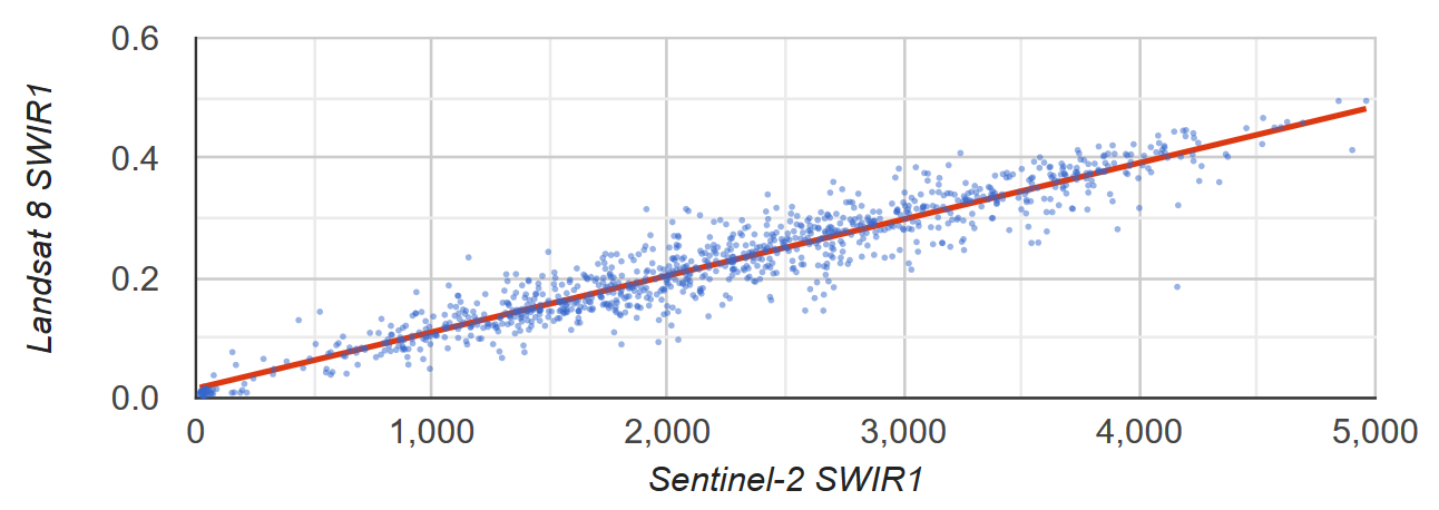
รูปที่ 2 ผังกระจายและเส้นหาค่าสัมประสิทธิ์การถดถอยเชิงเส้นด้วยวิธีอย่างน้อยที่สุดสำหรับตัวอย่างพิกเซลที่แสดงการสะท้อนแสง TOA ของ SWIR1 จาก Sentinel-2 และ Landsat 8

ee.List

คอลัมน์ของออบเจ็กต์ ee.List 2 มิติสามารถใช้เป็นอินพุตสำหรับตัวลดขนาดการหาค่าประมาณได้ ตัวอย่างต่อไปนี้เป็นหลักฐานง่ายๆ ตัวแปรอิสระคือสําเนาของตัวแปรตามซึ่งให้ค่าตัดแกน y เท่ากับ 0 และค่าความชันเท่ากับ 1

`linearFit()`

เครื่องมือแก้ไขโค้ด (JavaScript)

// Define a list of lists, where columns represent variables. The first column
// is the independent variable and the second is the dependent variable.
var listsVarColumns = ee.List([
  [1, 1],
  [2, 2],
  [3, 3],
  [4, 4],
  [5, 5]
]);

// Compute the least squares estimate of a linear function. Note that an
// object is returned; cast it as an ee.Dictionary to make accessing the
// coefficients easier.
var linearFit = ee.Dictionary(listsVarColumns.reduce(ee.Reducer.linearFit()));

// Inspect the result.
print(linearFit);
print('y-intercept:', linearFit.get('offset'));
print('Slope:', linearFit.get('scale'));

เปลี่ยนรูปแบบรายการหากตัวแปรแสดงด้วยแถวโดยแปลงเป็น ee.Array แล้วเปลี่ยนรูปแบบ จากนั้นแปลงกลับเป็น ee.List

เครื่องมือแก้ไขโค้ด (JavaScript)

// If variables in the list are arranged as rows, you'll need to transpose it.
// Define a list of lists where rows represent variables. The first row is the
// independent variable and the second is the dependent variable.
var listsVarRows = ee.List([
  [1, 2, 3, 4, 5],
  [1, 2, 3, 4, 5]
]);

// Cast the ee.List as an ee.Array, transpose it, and cast back to ee.List.
var listsVarColumns = ee.Array(listsVarRows).transpose().toList();

// Compute the least squares estimate of a linear function. Note that an
// object is returned; cast it as an ee.Dictionary to make accessing the
// coefficients easier.
var linearFit = ee.Dictionary(listsVarColumns.reduce(ee.Reducer.linearFit()));

// Inspect the result.
print(linearFit);
print('y-intercept:', linearFit.get('offset'));
print('Slope:', linearFit.get('scale'));

`linearRegression()`

การใช้งาน ee.Reducer.linearRegression() คล้ายกับตัวอย่าง linearFit() ด้านบน ยกเว้นว่ามีตัวแปรอิสระแบบคงที่รวมอยู่ด้วย

เครื่องมือแก้ไขโค้ด (JavaScript)

// Define a list of lists where columns represent variables. The first column
// represents a constant term, the second an independent variable, and the third
// a dependent variable.
var listsVarColumns = ee.List([
  [1, 1, 1],
  [1, 2, 2],
  [1, 3, 3],
  [1, 4, 4],
  [1, 5, 5]
]);

// Compute ordinary least squares regression coefficients. numX is 2 because
// there is one constant term and an additional independent variable. numY is 1
// because there is only a single dependent variable. Cast the resulting
// object to an ee.Dictionary for easy access to the properties.
var linearRegression = ee.Dictionary(
  listsVarColumns.reduce(ee.Reducer.linearRegression({
    numX: 2,
    numY: 1
})));

// Convert the coefficients array to a list.
var coefList = ee.Array(linearRegression.get('coefficients')).toList();

// Extract the y-intercept and slope.
var b0 = ee.List(coefList.get(0)).get(0); // y-intercept
var b1 = ee.List(coefList.get(1)).get(0); // slope

// Extract the residuals.
var residuals = ee.Array(linearRegression.get('residuals')).toList().get(0);

// Inspect the results.
print('OLS estimates', linearRegression);
print('y-intercept:', b0);
print('Slope:', b1);
print('Residuals:', residuals);