Doğrusal Regresyon

Earth Engine, azaltıcılar kullanarak doğrusal regresyon gerçekleştirmek için çeşitli yöntemlere sahiptir:

• ee.Reducer.linearFit()
• ee.Reducer.linearRegression()
• ee.Reducer.robustLinearRegression()
• ee.Reducer.ridgeRegression()

En basit doğrusal regresyon azaltıcı, sabit terimli bir değişkenin doğrusal fonksiyonunun en küçük kare tahminini hesaplayan linearFit()'tür. Doğrusal modellemeye daha esnek bir yaklaşım için değişken sayıda bağımsız ve bağımlı değişkene izin veren doğrusal regresyon azaltıcılardan birini kullanın. linearRegression(), sıradan en küçük kareler regresyonunu(OLS) uygular. robustLinearRegression(), verilerdeki aykırı değerlerin ağırlığını iteratif olarak azaltmak için regresyon artıklarına dayalı bir maliyet işlevi kullanır (O’Leary, 1990). ridgeRegression(), L2 normalleştirmesi ile doğrusal regresyon yapar.

Bu yöntemlerle regresyon analizi, ee.ImageCollection, ee.Image, ee.FeatureCollection ve ee.List nesnelerini azaltmak için uygundur. Aşağıdaki örneklerde her biri için bir uygulama gösterilmektedir. linearRegression(), robustLinearRegression() ve ridgeRegression()'nin aynı giriş ve çıkış yapılarına sahip olduğunu, ancak linearFit()'ın iki bantlı bir giriş (X ve ardından Y) beklediğini ve ridgeRegression()'nin ek bir parametresi (lambda, isteğe bağlı) ve çıkışı (pValue) olduğunu unutmayın.

Not: matrixSolve(), en küçük kareler regresyonu için ee.Reducer olarak uygulanmayan alternatif bir yöntem sağlar.

ee.ImageCollection

linearFit()

Veriler, ilk bant bağımsız değişken, ikinci bant ise bağımlı değişken olacak şekilde iki bantlı bir giriş resmi olarak ayarlanmalıdır. Aşağıdaki örnekte, iklim modelleri tarafından öngörülen gelecekteki yağışların doğrusal eğiliminin (NEX-DCP30 verilerinde 2006'dan sonra) tahmini gösterilmektedir. Bağımlı değişken, tahmini yağış miktarı, bağımsız değişken ise linearFit() çağrılmadan önce eklenen zamandır:

Kod Düzenleyici (JavaScript)

// This function adds a time band to the image.
var createTimeBand = function(image) {
  // Scale milliseconds by a large constant to avoid very small slopes
  // in the linear regression output.
  return image.addBands(image.metadata('system:time_start').divide(1e18));
};

// Load the input image collection: projected climate data.
var collection = ee.ImageCollection('NASA/NEX-DCP30_ENSEMBLE_STATS')
  .filter(ee.Filter.eq('scenario', 'rcp85'))
  .filterDate(ee.Date('2006-01-01'), ee.Date('2050-01-01'))
  // Map the time band function over the collection.
  .map(createTimeBand);

// Reduce the collection with the linear fit reducer.
// Independent variable are followed by dependent variables.
var linearFit = collection.select(['system:time_start', 'pr_mean'])
  .reduce(ee.Reducer.linearFit());

// Display the results.
Map.setCenter(-100.11, 40.38, 5);
Map.addLayer(linearFit,
  {min: 0, max: [-0.9, 8e-5, 1], bands: ['scale', 'offset', 'scale']}, 'fit');

Çıktının "ofset" (kesme noktası) ve "ölçek" olmak üzere iki bant içerdiğini görebilirsiniz ("ölçek" bu bağlamda çizginin eğimini ifade eder ve birçok azaltıcıya girilen ölçek parametresi (uzamsal ölçek) ile karıştırılmamalıdır). Artış trendi olan alanlar mavi, düşüş trendi olan alanlar kırmızı ve trend olmayan alanlar yeşil renkte olacak şekilde elde edilen sonuç Şekil 1'e benzer şekilde görünür.

Şekil 1. Tahmini yağışa uygulanan linearFit() sonucu. Yağış miktarının artacağı tahmin edilen bölgeler mavi, azalacağı tahmin edilen bölgeler ise kırmızı renkle gösterilir.

linearRegression()

Örneğin, iki bağımlı değişken (yağış ve maksimum sıcaklık) ve iki bağımsız değişken (sabit ve zaman) olduğunu varsayalım. Koleksiyon önceki örneğe benzer ancak sabit bant, azaltmadan önce manuel olarak eklenmelidir. Girişin ilk iki bandı "X" (bağımsız) değişkenler, sonraki iki band ise "Y" (bağımlı) değişkenlerdir. Bu örnekte, önce regresyon katsayılarını alın, ardından ilgilendiğiniz bantları ayıklamak için dizi resmini düzleştirin:

Kod Düzenleyici (JavaScript)

// This function adds a time band to the image.
var createTimeBand = function(image) {
  // Scale milliseconds by a large constant.
  return image.addBands(image.metadata('system:time_start').divide(1e18));
};

// This function adds a constant band to the image.
var createConstantBand = function(image) {
  return ee.Image(1).addBands(image);
};

// Load the input image collection: projected climate data.
var collection = ee.ImageCollection('NASA/NEX-DCP30_ENSEMBLE_STATS')
  .filterDate(ee.Date('2006-01-01'), ee.Date('2099-01-01'))
  .filter(ee.Filter.eq('scenario', 'rcp85'))
  // Map the functions over the collection, to get constant and time bands.
  .map(createTimeBand)
  .map(createConstantBand)
  // Select the predictors and the responses.
  .select(['constant', 'system:time_start', 'pr_mean', 'tasmax_mean']);

// Compute ordinary least squares regression coefficients.
var linearRegression = collection.reduce(
  ee.Reducer.linearRegression({
    numX: 2,
    numY: 2
}));

// Compute robust linear regression coefficients.
var robustLinearRegression = collection.reduce(
  ee.Reducer.robustLinearRegression({
    numX: 2,
    numY: 2
}));

// The results are array images that must be flattened for display.
// These lists label the information along each axis of the arrays.
var bandNames = [['constant', 'time'], // 0-axis variation.
                 ['precip', 'temp']]; // 1-axis variation.

// Flatten the array images to get multi-band images according to the labels.
var lrImage = linearRegression.select(['coefficients']).arrayFlatten(bandNames);
var rlrImage = robustLinearRegression.select(['coefficients']).arrayFlatten(bandNames);

// Display the OLS results.
Map.setCenter(-100.11, 40.38, 5);
Map.addLayer(lrImage,
  {min: 0, max: [-0.9, 8e-5, 1], bands: ['time_precip', 'constant_precip', 'time_precip']}, 'OLS');

// Compare the results at a specific point:
print('OLS estimates:', lrImage.reduceRegion({
  reducer: ee.Reducer.first(),
  geometry: ee.Geometry.Point([-96.0, 41.0]),
  scale: 1000
}));

print('Robust estimates:', rlrImage.reduceRegion({
  reducer: ee.Reducer.first(),
  geometry: ee.Geometry.Point([-96.0, 41.0]),
  scale: 1000
}));

linearRegression() çıkışının, linearFit() azaltıcısı tarafından tahmin edilen katsayılara eşdeğer olduğunu keşfetmek için sonuçları inceleyin. Ancak linearRegression() çıkışında diğer bağımlı değişken tasmax_mean için de katsayılar vardır. Güçlü doğrusal regresyon katsayıları, OLS tahminlerinden farklıdır. Örnekte, belirli bir noktada farklı regresyon yöntemlerinden elde edilen katsayılar karşılaştırılmaktadır.

ee.Image

ee.Image nesnesi bağlamında, bölgelerdeki piksellerde doğrusal regresyon gerçekleştirmek için regresyon azaltıcılar reduceRegion veya reduceRegions ile kullanılabilir. Aşağıdaki örneklerde, rastgele bir poligondaki Landsat bantları arasındaki regresyon katsayılarının nasıl hesaplanacağı gösterilmektedir.

linearFit()

Dizi veri grafiklerini açıklayan kılavuz bölümünde, Landsat 8 SWIR1 ve SWIR2 bantları arasındaki korelasyona ait bir dağılım grafiği gösterilmektedir. Burada, bu ilişki için doğrusal regresyon katsayıları hesaplanır. 'offset' (y kesme noktası) ve 'scale' (eğim) özelliklerini içeren bir sözlük döndürülür.

Kod Düzenleyici (JavaScript)

// Define a rectangle geometry around San Francisco.
var sanFrancisco = ee.Geometry.Rectangle([-122.45, 37.74, -122.4, 37.8]);

// Import a Landsat 8 TOA image for this region.
var img = ee.Image('LANDSAT/LC08/C02/T1_TOA/LC08_044034_20140318');

// Subset the SWIR1 and SWIR2 bands. In the regression reducer, independent
// variables come first followed by the dependent variables. In this case,
// B5 (SWIR1) is the independent variable and B6 (SWIR2) is the dependent
// variable.
var imgRegress = img.select(['B5', 'B6']);

// Calculate regression coefficients for the set of pixels intersecting the
// above defined region using reduceRegion with ee.Reducer.linearFit().
var linearFit = imgRegress.reduceRegion({
  reducer: ee.Reducer.linearFit(),
  geometry: sanFrancisco,
  scale: 30,
});

// Inspect the results.
print('OLS estimates:', linearFit);
print('y-intercept:', linearFit.get('offset'));
print('Slope:', linearFit.get('scale'));

linearRegression()

Önceki linearFit bölümündeki aynı analiz burada da uygulanır. Tek fark, bu kez ee.Reducer.linearRegression işlevinin kullanılmasıdır. Regresyon görüntüsünün üç ayrı görüntüden oluştuğunu unutmayın: Sabit bir görüntü ve aynı Landsat 8 görüntüsünden SWIR1 ve SWIR2 bantlarını temsil eden görüntüler. ee.Reducer.linearRegression tarafından bölge azaltma için bir giriş resmi oluşturmak üzere herhangi bir bant grubunu birleştirebileceğinizi unutmayın. Bu bantların aynı kaynak görüntüye ait olması gerekmez.

Kod Düzenleyici (JavaScript)

// Define a rectangle geometry around San Francisco.
var sanFrancisco = ee.Geometry.Rectangle([-122.45, 37.74, -122.4, 37.8]);

// Import a Landsat 8 TOA image for this region.
var img = ee.Image('LANDSAT/LC08/C02/T1_TOA/LC08_044034_20140318');

// Create a new image that is the concatenation of three images: a constant,
// the SWIR1 band, and the SWIR2 band.
var constant = ee.Image(1);
var xVar = img.select('B5');
var yVar = img.select('B6');
var imgRegress = ee.Image.cat(constant, xVar, yVar);

// Calculate regression coefficients for the set of pixels intersecting the
// above defined region using reduceRegion. The numX parameter is set as 2
// because the constant and the SWIR1 bands are independent variables and they
// are the first two bands in the stack; numY is set as 1 because there is only
// one dependent variable (SWIR2) and it follows as band three in the stack.
var linearRegression = imgRegress.reduceRegion({
  reducer: ee.Reducer.linearRegression({
    numX: 2,
    numY: 1
  }),
  geometry: sanFrancisco,
  scale: 30,
});

// Convert the coefficients array to a list.
var coefList = ee.Array(linearRegression.get('coefficients')).toList();

// Extract the y-intercept and slope.
var b0 = ee.List(coefList.get(0)).get(0); // y-intercept
var b1 = ee.List(coefList.get(1)).get(0); // slope

// Extract the residuals.
var residuals = ee.Array(linearRegression.get('residuals')).toList().get(0);

// Inspect the results.
print('OLS estimates', linearRegression);
print('y-intercept:', b0);
print('Slope:', b1);
print('Residuals:', residuals);

'coefficients' ve 'residuals' özelliklerini içeren bir sözlük döndürülür. 'coefficients' mülkü, boyutları (numX, numY) olan bir dizidir; her sütun, ilgili bağımlı değişkenin katsayılarını içerir. Bu örnekte dizi iki satır ve bir sütundan oluşur. Birinci satır, birinci sütun y kesme noktası, ikinci satır, birinci sütun ise eğimdir. 'residuals' mülkü, her bağımlı değişkenin artıklarının karekökü ortalamasının vektörüdür. Sonuçları dizi olarak yayınlayıp ardından istediğiniz öğeleri dilimleyerek veya diziyi listeye dönüştürüp katsayıları dizin konumuna göre seçerek katsayıları ayıklayın.

ee.FeatureCollection

Sentinel-2 ile Landsat 8 SWIR1 yansıması arasındaki doğrusal ilişkiyi öğrenmek istediğinizi varsayalım. Bu örnekte, ilişkiyi hesaplamak için noktaların özellik koleksiyonu olarak biçimlendirilmiş rastgele bir piksel örneği kullanılır. En küçük kareler en iyi uyum çizgisiyle birlikte piksel çiftlerinin dağılım grafiği oluşturulur (Şekil 2).

Kod Düzenleyici (JavaScript)

// Import a Sentinel-2 TOA image.
var s2ImgSwir1 = ee.Image('COPERNICUS/S2/20191022T185429_20191022T185427_T10SEH');

// Import a Landsat 8 TOA image from 12 days earlier than the S2 image.
var l8ImgSwir1 = ee.Image('LANDSAT/LC08/C02/T1_TOA/LC08_044033_20191010');

// Get the intersection between the two images - the area of interest (aoi).
var aoi = s2ImgSwir1.geometry().intersection(l8ImgSwir1.geometry());

// Get a set of 1000 random points from within the aoi. A feature collection
// is returned.
var sample = ee.FeatureCollection.randomPoints({
  region: aoi,
  points: 1000
});

// Combine the SWIR1 bands from each image into a single image.
var swir1Bands = s2ImgSwir1.select('B11')
  .addBands(l8ImgSwir1.select('B6'))
  .rename(['s2_swir1', 'l8_swir1']);

// Sample the SWIR1 bands using the sample point feature collection.
var imgSamp = swir1Bands.sampleRegions({
  collection: sample,
  scale: 30
})
// Add a constant property to each feature to be used as an independent variable.
.map(function(feature) {
  return feature.set('constant', 1);
});

// Compute linear regression coefficients. numX is 2 because
// there are two independent variables: 'constant' and 's2_swir1'. numY is 1
// because there is a single dependent variable: 'l8_swir1'. Cast the resulting
// object to an ee.Dictionary for easy access to the properties.
var linearRegression = ee.Dictionary(imgSamp.reduceColumns({
  reducer: ee.Reducer.linearRegression({
    numX: 2,
    numY: 1
  }),
  selectors: ['constant', 's2_swir1', 'l8_swir1']
}));

// Convert the coefficients array to a list.
var coefList = ee.Array(linearRegression.get('coefficients')).toList();

// Extract the y-intercept and slope.
var yInt = ee.List(coefList.get(0)).get(0); // y-intercept
var slope = ee.List(coefList.get(1)).get(0); // slope

// Gather the SWIR1 values from the point sample into a list of lists.
var props = ee.List(['s2_swir1', 'l8_swir1']);
var regressionVarsList = ee.List(imgSamp.reduceColumns({
  reducer: ee.Reducer.toList().repeat(props.size()),
  selectors: props
}).get('list'));

// Convert regression x and y variable lists to an array - used later as input
// to ui.Chart.array.values for generating a scatter plot.
var x = ee.Array(ee.List(regressionVarsList.get(0)));
var y1 = ee.Array(ee.List(regressionVarsList.get(1)));

// Apply the line function defined by the slope and y-intercept of the
// regression to the x variable list to create an array that will represent
// the regression line in the scatter plot.
var y2 = ee.Array(ee.List(regressionVarsList.get(0)).map(function(x) {
  var y = ee.Number(x).multiply(slope).add(yInt);
  return y;
}));

// Concatenate the y variables (Landsat 8 SWIR1 and predicted y) into an array
// for input to ui.Chart.array.values for plotting a scatter plot.
var yArr = ee.Array.cat([y1, y2], 1);

// Make a scatter plot of the two SWIR1 bands for the point sample and include
// the least squares line of best fit through the data.
print(ui.Chart.array.values({
  array: yArr,
  axis: 0,
  xLabels: x})
  .setChartType('ScatterChart')
  .setOptions({
    legend: {position: 'none'},
    hAxis: {'title': 'Sentinel-2 SWIR1'},
    vAxis: {'title': 'Landsat 8 SWIR1'},
    series: {
      0: {
        pointSize: 0.2,
        dataOpacity: 0.5,
      },
      1: {
        pointSize: 0,
        lineWidth: 2,
      }
    }
  })
);

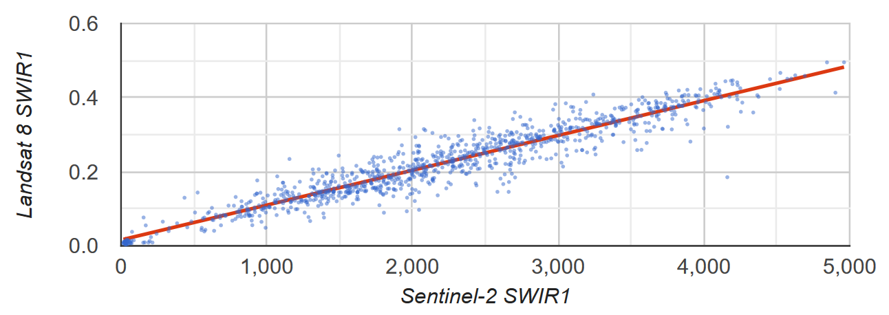
Şekil 2. Sentinel-2 ve Landsat 8 SWIR1 TOA yansımasını temsil eden bir piksel örneği için dağılım grafiği ve en küçük kareler doğrusal regresyon çizgisi.

ee.List

2 boyutlu ee.List nesnelerinin sütunları, regresyon azaltıcılara giriş olabilir. Aşağıdaki örneklerde basit kanıtlar verilmiştir. Bağımsız değişken, 0'a eşit bir y kesme noktası ve 1'e eşit bir eğim oluşturan bağımlı değişkenin bir kopyasıdır.

Not: ee.List azaltma işleminin sonucunun bir nesne olduğunu unutmayın. Özelliklere erişimi kolaylaştırmak için bir ee.Dictionary olarak yayınlayabilirsiniz.

Dikkat: Satırlar ve sütunlar arasındaki uzunluklar eşit olmalıdır. Eksik veri girişlerini temsil etmek için null kullanın.

linearFit()

Kod Düzenleyici (JavaScript)

// Define a list of lists, where columns represent variables. The first column
// is the independent variable and the second is the dependent variable.
var listsVarColumns = ee.List([
  [1, 1],
  [2, 2],
  [3, 3],
  [4, 4],
  [5, 5]
]);

// Compute the least squares estimate of a linear function. Note that an
// object is returned; cast it as an ee.Dictionary to make accessing the
// coefficients easier.
var linearFit = ee.Dictionary(listsVarColumns.reduce(ee.Reducer.linearFit()));

// Inspect the result.
print(linearFit);
print('y-intercept:', linearFit.get('offset'));
print('Slope:', linearFit.get('scale'));

ee.Array olarak dönüştürüp transpoze ettikten sonra tekrar ee.List olarak dönüştürerek değişkenler satırlarla temsil ediliyorsa listeyi transpoze edin.

Kod Düzenleyici (JavaScript)

// If variables in the list are arranged as rows, you'll need to transpose it.
// Define a list of lists where rows represent variables. The first row is the
// independent variable and the second is the dependent variable.
var listsVarRows = ee.List([
  [1, 2, 3, 4, 5],
  [1, 2, 3, 4, 5]
]);

// Cast the ee.List as an ee.Array, transpose it, and cast back to ee.List.
var listsVarColumns = ee.Array(listsVarRows).transpose().toList();

// Compute the least squares estimate of a linear function. Note that an
// object is returned; cast it as an ee.Dictionary to make accessing the
// coefficients easier.
var linearFit = ee.Dictionary(listsVarColumns.reduce(ee.Reducer.linearFit()));

// Inspect the result.
print(linearFit);
print('y-intercept:', linearFit.get('offset'));
print('Slope:', linearFit.get('scale'));

linearRegression()

ee.Reducer.linearRegression()'ün uygulanması, sabit bir bağımsız değişkenin dahil edilmesi dışında yukarıdaki linearFit() örneğine benzer.

Kod Düzenleyici (JavaScript)

// Define a list of lists where columns represent variables. The first column
// represents a constant term, the second an independent variable, and the third
// a dependent variable.
var listsVarColumns = ee.List([
  [1, 1, 1],
  [1, 2, 2],
  [1, 3, 3],
  [1, 4, 4],
  [1, 5, 5]
]);

// Compute ordinary least squares regression coefficients. numX is 2 because
// there is one constant term and an additional independent variable. numY is 1
// because there is only a single dependent variable. Cast the resulting
// object to an ee.Dictionary for easy access to the properties.
var linearRegression = ee.Dictionary(
  listsVarColumns.reduce(ee.Reducer.linearRegression({
    numX: 2,
    numY: 1
})));

// Convert the coefficients array to a list.
var coefList = ee.Array(linearRegression.get('coefficients')).toList();

// Extract the y-intercept and slope.
var b0 = ee.List(coefList.get(0)).get(0); // y-intercept
var b1 = ee.List(coefList.get(1)).get(0); // slope

// Extract the residuals.
var residuals = ee.Array(linearRegression.get('residuals')).toList().get(0);

// Inspect the results.
print('OLS estimates', linearRegression);
print('y-intercept:', b0);
print('Slope:', b1);
print('Residuals:', residuals);