Earth Engine 提供多種方法,可使用減法器執行線性迴歸:
ee.Reducer.linearFit()ee.Reducer.linearRegression()ee.Reducer.robustLinearRegression()ee.Reducer.ridgeRegression()
最簡單的線性迴歸縮減器是 linearFit(),可計算單一變數線性函數的常數項最小平方估計值。如要採用更靈活的線性建模方法,請使用其中一個線性迴歸縮減器,允許變數數量的獨立和從屬變數。linearRegression() 會實作一般最小平方迴歸法(OLS)。robustLinearRegression() 會使用以迴歸殘差為基礎的成本函式,以便逐步降低資料中的異常值權重 (O’Leary, 1990)。ridgeRegression() 會使用 L2 正則化進行線性迴歸。
使用這些方法進行迴歸分析,適合用於減少 ee.ImageCollection、ee.Image、ee.FeatureCollection 和 ee.List 物件。以下範例說明每個類型的應用程式。請注意,linearRegression()、robustLinearRegression() 和 ridgeRegression() 都具有相同的輸入和輸出結構,但 linearFit() 預期會收到雙頻帶輸入內容 (X 後面接著 Y),而 ridgeRegression() 則有額外的參數 (lambda,選用) 和輸出內容 (pValue)。
ee.ImageCollection
linearFit()
資料應設為雙頻帶輸入圖片,其中第一個頻帶是獨立變數,第二個頻帶是相依變數。以下範例顯示氣候模型預測的未來降雨量線性趨勢 (NEX-DCP30 資料 中 2006 年後的資料)。相依變數是預估降雨量,獨立變數則是時間,這兩個變數會在呼叫 linearFit() 之前新增:
程式碼編輯器 (JavaScript)
// This function adds a time band to the image.
var createTimeBand = function(image) {
  // Scale milliseconds by a large constant to avoid very small slopes
  // in the linear regression output.
  return image.addBands(image.metadata('system:time_start').divide(1e18));
};

// Load the input image collection: projected climate data.
var collection = ee.ImageCollection('NASA/NEX-DCP30_ENSEMBLE_STATS')
  .filter(ee.Filter.eq('scenario', 'rcp85'))
  .filterDate(ee.Date('2006-01-01'), ee.Date('2050-01-01'))
  // Map the time band function over the collection.
  .map(createTimeBand);

// Reduce the collection with the linear fit reducer.
// Independent variable are followed by dependent variables.
var linearFit = collection.select(['system:time_start', 'pr_mean'])
  .reduce(ee.Reducer.linearFit());

// Display the results.
Map.setCenter(-100.11, 40.38, 5);
Map.addLayer(linearFit,
  {min: 0, max: [-0.9, 8e-5, 1], bands: ['scale', 'offset', 'scale']}, 'fit');
請注意,輸出內容包含兩個頻帶:「偏移」(截距) 和「比例」(在此情況下是指線的斜率,請勿與輸入至多個縮減器的比例參數混淆,後者是空間比例)。結果會顯示藍色區域代表趨勢上升、紅色區域代表趨勢下降,而綠色區域代表沒有趨勢,如圖 1 所示。
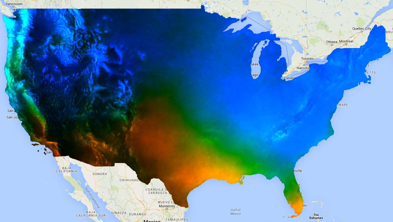
圖 1. linearFit() 的輸出內容已套用至預估降雨量。預測降雨量增加的區域會以藍色顯示,降雨量減少的區域則會以紅色顯示。
linearRegression()
舉例來說,假設有兩個從屬變數:降雨量和最高溫度,以及兩個獨立變數:常數和時間。集合與前一個範例相同,但必須在縮減前手動新增常數頻帶。輸入內容的前兩個頻帶是「X」(獨立) 變數,後兩個頻帶則是「Y」(相依) 變數。在本例中,您會先取得迴歸係數,然後將陣列圖片平坦化,以便擷取感興趣的頻帶:
程式碼編輯器 (JavaScript)
// This function adds a time band to the image.
var createTimeBand = function(image) {
  // Scale milliseconds by a large constant.
  return image.addBands(image.metadata('system:time_start').divide(1e18));
};

// This function adds a constant band to the image.
var createConstantBand = function(image) {
  return ee.Image(1).addBands(image);
};

// Load the input image collection: projected climate data.
var collection = ee.ImageCollection('NASA/NEX-DCP30_ENSEMBLE_STATS')
  .filterDate(ee.Date('2006-01-01'), ee.Date('2099-01-01'))
  .filter(ee.Filter.eq('scenario', 'rcp85'))
  // Map the functions over the collection, to get constant and time bands.
  .map(createTimeBand)
  .map(createConstantBand)
  // Select the predictors and the responses.
  .select(['constant', 'system:time_start', 'pr_mean', 'tasmax_mean']);

// Compute ordinary least squares regression coefficients.
var linearRegression = collection.reduce(
  ee.Reducer.linearRegression({
    numX: 2,
    numY: 2
}));

// Compute robust linear regression coefficients.
var robustLinearRegression = collection.reduce(
  ee.Reducer.robustLinearRegression({
    numX: 2,
    numY: 2
}));

// The results are array images that must be flattened for display.
// These lists label the information along each axis of the arrays.
var bandNames = [['constant', 'time'], // 0-axis variation.
                 ['precip', 'temp']]; // 1-axis variation.

// Flatten the array images to get multi-band images according to the labels.
var lrImage = linearRegression.select(['coefficients']).arrayFlatten(bandNames);
var rlrImage = robustLinearRegression.select(['coefficients']).arrayFlatten(bandNames);

// Display the OLS results.
Map.setCenter(-100.11, 40.38, 5);
Map.addLayer(lrImage,
  {min: 0, max: [-0.9, 8e-5, 1], bands: ['time_precip', 'constant_precip', 'time_precip']}, 'OLS');

// Compare the results at a specific point:
print('OLS estimates:', lrImage.reduceRegion({
  reducer: ee.Reducer.first(),
  geometry: ee.Geometry.Point([-96.0, 41.0]),
  scale: 1000
}));

print('Robust estimates:', rlrImage.reduceRegion({
  reducer: ee.Reducer.first(),
  geometry: ee.Geometry.Point([-96.0, 41.0]),
  scale: 1000
}));
檢查結果,即可發現 linearRegression() 輸出結果等同於 linearFit() 縮減器估算的係數,但 linearRegression() 輸出結果也包含其他依附變數 tasmax_mean 的係數。穩健線性迴歸係數與 OLS 估計值不同。本範例會比較不同迴歸方法在特定時間點的係數。
ee.Image
在 ee.Image 物件的內容中,您可以搭配使用迴歸縮減器和 reduceRegion 或 reduceRegions,針對區域中的像素執行線性迴歸。以下範例說明如何計算任意多邊形內 Landsat 波段之間的迴歸係數。
linearFit()
說明陣列資料圖表的指南章節中,顯示了 Landsat 8 SWIR1 和 SWIR2 頻帶之間關聯性的散布圖。此處會計算此關係的線性迴歸係數。系統會傳回字典,其中包含 'offset' (y 軸交點) 和 'scale' (斜率) 屬性。
程式碼編輯器 (JavaScript)
// Define a rectangle geometry around San Francisco.
var sanFrancisco = ee.Geometry.Rectangle([-122.45, 37.74, -122.4, 37.8]);

// Import a Landsat 8 TOA image for this region.
var img = ee.Image('LANDSAT/LC08/C02/T1_TOA/LC08_044034_20140318');

// Subset the SWIR1 and SWIR2 bands. In the regression reducer, independent
// variables come first followed by the dependent variables. In this case,
// B5 (SWIR1) is the independent variable and B6 (SWIR2) is the dependent
// variable.
var imgRegress = img.select(['B5', 'B6']);

// Calculate regression coefficients for the set of pixels intersecting the
// above defined region using reduceRegion with ee.Reducer.linearFit().
var linearFit = imgRegress.reduceRegion({
  reducer: ee.Reducer.linearFit(),
  geometry: sanFrancisco,
  scale: 30,
});

// Inspect the results.
print('OLS estimates:', linearFit);
print('y-intercept:', linearFit.get('offset'));
print('Slope:', linearFit.get('scale'));
linearRegression()
這裡會套用先前 linearFit 部分的相同分析,但這次會使用 ee.Reducer.linearRegression 函式。請注意,回歸圖片是由三張獨立圖片建構而成:一張常數圖片,以及代表同一張 Landsat 8 圖片的 SWIR1 和 SWIR2 頻帶圖片。請注意,您可以結合任何一組頻帶,透過 ee.Reducer.linearRegression 建構用於區域縮減的輸入圖像,這些頻帶不必屬於相同的來源圖像。
程式碼編輯器 (JavaScript)
// Define a rectangle geometry around San Francisco.
var sanFrancisco = ee.Geometry.Rectangle([-122.45, 37.74, -122.4, 37.8]);

// Import a Landsat 8 TOA image for this region.
var img = ee.Image('LANDSAT/LC08/C02/T1_TOA/LC08_044034_20140318');

// Create a new image that is the concatenation of three images: a constant,
// the SWIR1 band, and the SWIR2 band.
var constant = ee.Image(1);
var xVar = img.select('B5');
var yVar = img.select('B6');
var imgRegress = ee.Image.cat(constant, xVar, yVar);

// Calculate regression coefficients for the set of pixels intersecting the
// above defined region using reduceRegion. The numX parameter is set as 2
// because the constant and the SWIR1 bands are independent variables and they
// are the first two bands in the stack; numY is set as 1 because there is only
// one dependent variable (SWIR2) and it follows as band three in the stack.
var linearRegression = imgRegress.reduceRegion({
  reducer: ee.Reducer.linearRegression({
    numX: 2,
    numY: 1
  }),
  geometry: sanFrancisco,
  scale: 30,
});

// Convert the coefficients array to a list.
var coefList = ee.Array(linearRegression.get('coefficients')).toList();

// Extract the y-intercept and slope.
var b0 = ee.List(coefList.get(0)).get(0); // y-intercept
var b1 = ee.List(coefList.get(1)).get(0); // slope

// Extract the residuals.
var residuals = ee.Array(linearRegression.get('residuals')).toList().get(0);

// Inspect the results.
print('OLS estimates', linearRegression);
print('y-intercept:', b0);
print('Slope:', b1);
print('Residuals:', residuals);
系統會傳回包含 'coefficients' 和 'residuals' 屬性的字典。'coefficients' 屬性是具有 (numX, numY) 維度的陣列,每個資料欄都包含對應依附變數的係數。在本例中,陣列有兩列和一個欄;第一列第一欄是 y 截距,第二列第一欄是斜率。'residuals' 屬性是各個依附變數殘差的平方根均方向量。您可以將結果轉換為陣列,然後切片所需的元素,或將陣列轉換為清單,並依索引位置選取係數,藉此擷取係數。
ee.FeatureCollection
假設您想瞭解 Sentinel-2 和 Landsat 8 SWIR1 反射率之間的線性關係。在本例中,我們使用以點為特徵集合的隨機像素樣本,計算關係。系統會產生像素組成的散布圖,以及最小二乘式最佳擬合線 (圖 2)。
程式碼編輯器 (JavaScript)
// Import a Sentinel-2 TOA image.
var s2ImgSwir1 = ee.Image('COPERNICUS/S2/20191022T185429_20191022T185427_T10SEH');

// Import a Landsat 8 TOA image from 12 days earlier than the S2 image.
var l8ImgSwir1 = ee.Image('LANDSAT/LC08/C02/T1_TOA/LC08_044033_20191010');

// Get the intersection between the two images - the area of interest (aoi).
var aoi = s2ImgSwir1.geometry().intersection(l8ImgSwir1.geometry());

// Get a set of 1000 random points from within the aoi. A feature collection
// is returned.
var sample = ee.FeatureCollection.randomPoints({
  region: aoi,
  points: 1000
});

// Combine the SWIR1 bands from each image into a single image.
var swir1Bands = s2ImgSwir1.select('B11')
  .addBands(l8ImgSwir1.select('B6'))
  .rename(['s2_swir1', 'l8_swir1']);

// Sample the SWIR1 bands using the sample point feature collection.
var imgSamp = swir1Bands.sampleRegions({
  collection: sample,
  scale: 30
})
// Add a constant property to each feature to be used as an independent variable.
.map(function(feature) {
  return feature.set('constant', 1);
});

// Compute linear regression coefficients. numX is 2 because
// there are two independent variables: 'constant' and 's2_swir1'. numY is 1
// because there is a single dependent variable: 'l8_swir1'. Cast the resulting
// object to an ee.Dictionary for easy access to the properties.
var linearRegression = ee.Dictionary(imgSamp.reduceColumns({
  reducer: ee.Reducer.linearRegression({
    numX: 2,
    numY: 1
  }),
  selectors: ['constant', 's2_swir1', 'l8_swir1']
}));

// Convert the coefficients array to a list.
var coefList = ee.Array(linearRegression.get('coefficients')).toList();

// Extract the y-intercept and slope.
var yInt = ee.List(coefList.get(0)).get(0); // y-intercept
var slope = ee.List(coefList.get(1)).get(0); // slope

// Gather the SWIR1 values from the point sample into a list of lists.
var props = ee.List(['s2_swir1', 'l8_swir1']);
var regressionVarsList = ee.List(imgSamp.reduceColumns({
  reducer: ee.Reducer.toList().repeat(props.size()),
  selectors: props
}).get('list'));

// Convert regression x and y variable lists to an array - used later as input
// to ui.Chart.array.values for generating a scatter plot.
var x = ee.Array(ee.List(regressionVarsList.get(0)));
var y1 = ee.Array(ee.List(regressionVarsList.get(1)));

// Apply the line function defined by the slope and y-intercept of the
// regression to the x variable list to create an array that will represent
// the regression line in the scatter plot.
var y2 = ee.Array(ee.List(regressionVarsList.get(0)).map(function(x) {
  var y = ee.Number(x).multiply(slope).add(yInt);
  return y;
}));

// Concatenate the y variables (Landsat 8 SWIR1 and predicted y) into an array
// for input to ui.Chart.array.values for plotting a scatter plot.
var yArr = ee.Array.cat([y1, y2], 1);

// Make a scatter plot of the two SWIR1 bands for the point sample and include
// the least squares line of best fit through the data.
print(ui.Chart.array.values({
  array: yArr,
  axis: 0,
  xLabels: x})
  .setChartType('ScatterChart')
  .setOptions({
    legend: {position: 'none'},
    hAxis: {'title': 'Sentinel-2 SWIR1'},
    vAxis: {'title': 'Landsat 8 SWIR1'},
    series: {
      0: {
        pointSize: 0.2,
        dataOpacity: 0.5,
      },
      1: {
        pointSize: 0,
        lineWidth: 2,
      }
    }
  })
);
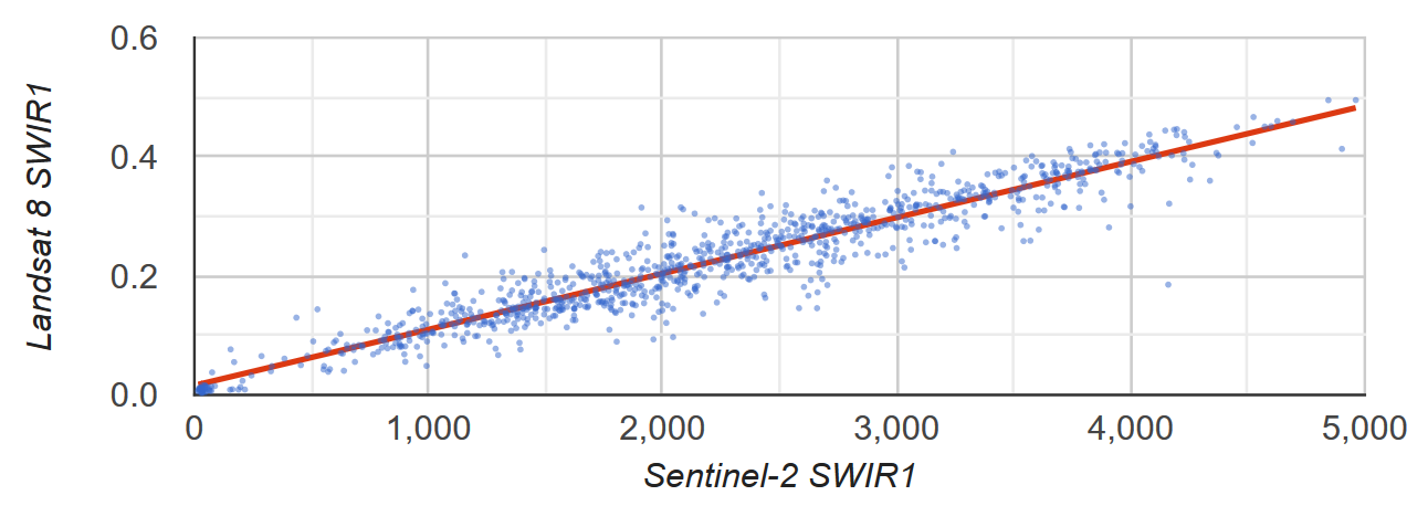
圖 2. 散布圖和最小平方迴歸線,代表 Sentinel-2 和 Landsat 8 SWIR1 TOA 反射率的像素樣本。
ee.List
2D ee.List 物件的欄可做為迴歸縮減器的輸入內容。以下範例提供簡單的證明;獨立變數是相依變數的副本,產生的 y 截距等於 0,斜率等於 1。
linearFit()
程式碼編輯器 (JavaScript)
// Define a list of lists, where columns represent variables. The first column
// is the independent variable and the second is the dependent variable.
var listsVarColumns = ee.List([
  [1, 1],
  [2, 2],
  [3, 3],
  [4, 4],
  [5, 5]
]);

// Compute the least squares estimate of a linear function. Note that an
// object is returned; cast it as an ee.Dictionary to make accessing the
// coefficients easier.
var linearFit = ee.Dictionary(listsVarColumns.reduce(ee.Reducer.linearFit()));

// Inspect the result.
print(linearFit);
print('y-intercept:', linearFit.get('offset'));
print('Slope:', linearFit.get('scale'));
如果變數以資料列表示,請將清單轉置,方法是將其轉換為 ee.Array、轉置,然後再轉換回 ee.List。
程式碼編輯器 (JavaScript)
// If variables in the list are arranged as rows, you'll need to transpose it.
// Define a list of lists where rows represent variables. The first row is the
// independent variable and the second is the dependent variable.
var listsVarRows = ee.List([
  [1, 2, 3, 4, 5],
  [1, 2, 3, 4, 5]
]);

// Cast the ee.List as an ee.Array, transpose it, and cast back to ee.List.
var listsVarColumns = ee.Array(listsVarRows).transpose().toList();

// Compute the least squares estimate of a linear function. Note that an
// object is returned; cast it as an ee.Dictionary to make accessing the
// coefficients easier.
var linearFit = ee.Dictionary(listsVarColumns.reduce(ee.Reducer.linearFit()));

// Inspect the result.
print(linearFit);
print('y-intercept:', linearFit.get('offset'));
print('Slope:', linearFit.get('scale'));
linearRegression()
ee.Reducer.linearRegression() 的應用方式與上述 linearFit() 範例類似,差別在於包含了常數獨立變數。
程式碼編輯器 (JavaScript)
// Define a list of lists where columns represent variables. The first column
// represents a constant term, the second an independent variable, and the third
// a dependent variable.
var listsVarColumns = ee.List([
  [1, 1, 1],
  [1, 2, 2],
  [1, 3, 3],
  [1, 4, 4],
  [1, 5, 5]
]);

// Compute ordinary least squares regression coefficients. numX is 2 because
// there is one constant term and an additional independent variable. numY is 1
// because there is only a single dependent variable. Cast the resulting
// object to an ee.Dictionary for easy access to the properties.
var linearRegression = ee.Dictionary(
  listsVarColumns.reduce(ee.Reducer.linearRegression({
    numX: 2,
    numY: 1
})));

// Convert the coefficients array to a list.
var coefList = ee.Array(linearRegression.get('coefficients')).toList();

// Extract the y-intercept and slope.
var b0 = ee.List(coefList.get(0)).get(0); // y-intercept
var b1 = ee.List(coefList.get(1)).get(0); // slope

// Extract the residuals.
var residuals = ee.Array(linearRegression.get('residuals')).toList().get(0);

// Inspect the results.
print('OLS estimates', linearRegression);
print('y-intercept:', b0);
print('Slope:', b1);
print('Residuals:', residuals);