דגימה מחדש והקטנת הרזולוציה

כפי שצוין במסמך תצוגות מפה, כברירת מחדל, Earth Engine מבצעת דגימה מחדש של השכן הקרוב ביותר במהלך הקרנת המפה מחדש. אפשר לשנות את ההתנהגות הזו באמצעות השיטות resample() או reduceResolution(). באופן ספציפי, כשחלה אחת מהשיטות האלה על תמונה של קלט, כל הקרנה מחדש הנדרשת של הקלט תתבצע באמצעות שיטת הדגימה מחדש או שיטת הצבירה שצוינה.

דגימה מחדש

הערך resample() גורם לשימוש בשיטת הדגימה מחדש שצוינה ('bilinear' או 'bicubic') בהקרנה מחדש הבאה. מכיוון שהבקשות להזנת נתונים מתבצעות בתוך הקרנה של הפלט, יכול להיות שקרנה מחדש משתמעת תתבצע לפני כל פעולה אחרת על הקלט. לכן, צריך להפעיל את resample() ישירות על תמונת הקלט. הנה דוגמה פשוטה:

Code Editor‏ (JavaScript)

// Load a Landsat image over San Francisco, California, UAS.
var landsat = ee.Image('LANDSAT/LC08/C02/T1_TOA/LC08_044034_20160323');

// Set display and visualization parameters.
Map.setCenter(-122.37383, 37.6193, 15);
var visParams = {bands: ['B4', 'B3', 'B2'], max: 0.3};

// Display the Landsat image using the default nearest neighbor resampling.
// when reprojecting to Mercator for the Code Editor map.
Map.addLayer(landsat, visParams, 'original image');

// Force the next reprojection on this image to use bicubic resampling.
var resampled = landsat.resample('bicubic');

// Display the Landsat image using bicubic resampling.
Map.addLayer(resampled, visParams, 'resampled');

הגדרת Python

בדף סביבת Python מפורט מידע על Python API ועל השימוש ב-geemap לפיתוח אינטראקטיבי.

import ee
import geemap.core as geemap

Colab (Python)

# Load a Landsat image over San Francisco, California, UAS.
landsat = ee.Image('LANDSAT/LC08/C02/T1_TOA/LC08_044034_20160323')

# Set display and visualization parameters.
m = geemap.Map()
m.set_center(-122.37383, 37.6193, 15)
vis_params = {'bands': ['B4', 'B3', 'B2'], 'max': 0.3}

# Display the Landsat image using the default nearest neighbor resampling.
# when reprojecting to Mercator for the Code Editor map.
m.add_layer(landsat, vis_params, 'original image')

# Force the next reprojection on this image to use bicubic resampling.
resampled = landsat.resample('bicubic')

# Display the Landsat image using bicubic resampling.
m.add_layer(resampled, vis_params, 'resampled')

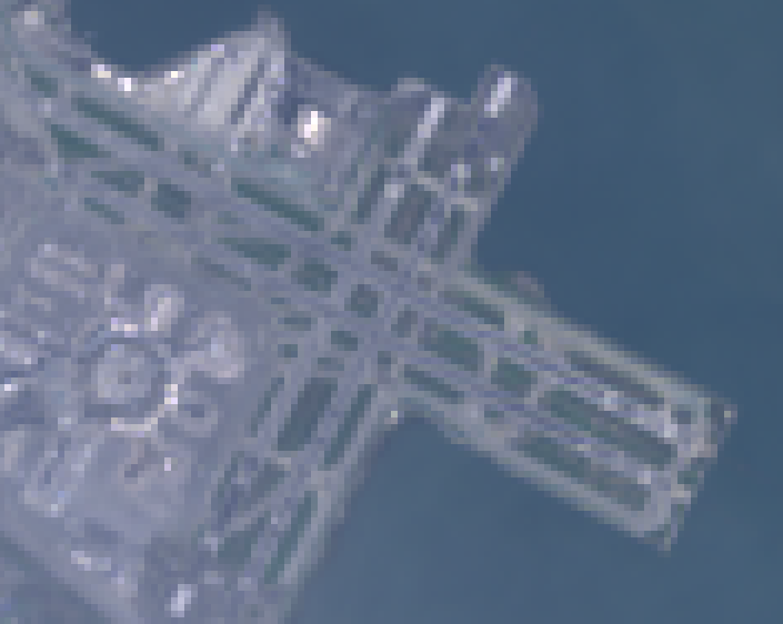
שימו לב: דגימת מחדש של 'bicubic' גורמת לכך שהפיקסלים של הפלט ייראו חלקים יותר בהשוואה לתמונה המקורית (איור 1).

איור 1א'. תמונות Landsat שעבר עליהן דגימה מחדש באמצעות שכן קרוב.

איור 1ב. תמונות Landsat שעברן דגימה מחדש באמצעות דגימה מחדש בינארית-קוביית.

סדר הפעולות בדוגמת הקוד הזו מתואר באיור 2. באופן ספציפי, ההיטל מחדש המשתמע להיטל maps Mercator מתבצע באמצעות שיטת הדגימה מחדש שצוינה בתמונה הקלט.

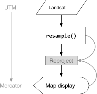
איור 2. תרשים תהליך של הפעולות כשמתבצעת קריאה ל-resample() בתמונה להזנה לפני ההצגה בעורך הקוד. הקווים המעוקלים מצביעים על זרימת המידע להקרנה מחדש: באופן ספציפי, הקרנת הפלט, קנה המידה והשיטה להחלפת דגימות.

הקטנת הרזולוציה

נניח שבמקום לדגום מחדש במהלך הקרנה מחדש, היעד שלכם הוא לצבור פיקסלים לפיקסלים גדולים יותר בתצוגה אחרת. האפשרות הזו שימושית כשמשווים בין קבוצות נתונים של תמונות בקנה מידה שונה, למשל פיקסלים של 30 מטר ממוצר שמבוסס על Landsat לעומת פיקסלים גסים (בקנה מידה גבוה יותר) ממוצר שמבוסס על MODIS. אפשר לשלוט בתהליך הצבירה הזה באמצעות השיטה reduceResolution(). בדומה ל-resample(), צריך לבצע קריאה ל-reduceResolution() על הקלט כדי להשפיע על הקרנת המשנה הבאה של התמונה. בדוגמה הבאה נעשה שימוש ב-reduceResolution() כדי להשוות בין נתוני כיסוי יערות ברזולוציה של 30 מטר לבין מדד צמחייה ברזולוציה של 500 מטר:

Code Editor‏ (JavaScript)

// Load a MODIS EVI image.
var modis = ee.Image(ee.ImageCollection('MODIS/061/MOD13A1').first())
    .select('EVI');

// Display the EVI image near La Honda, California.
Map.setCenter(-122.3616, 37.5331, 12);
Map.addLayer(modis, {min: 2000, max: 5000}, 'MODIS EVI');

// Get information about the MODIS projection.
var modisProjection = modis.projection();
print('MODIS projection:', modisProjection);

// Load and display forest cover data at 30 meters resolution.
var forest = ee.Image('UMD/hansen/global_forest_change_2023_v1_11')
    .select('treecover2000');
Map.addLayer(forest, {max: 80}, 'forest cover 30 m');

// Get the forest cover data at MODIS scale and projection.
var forestMean = forest
    // Force the next reprojection to aggregate instead of resampling.
    .reduceResolution({
      reducer: ee.Reducer.mean(),
      maxPixels: 1024
    })
    // Request the data at the scale and projection of the MODIS image.
    .reproject({
      crs: modisProjection
    });

// Display the aggregated, reprojected forest cover data.
Map.addLayer(forestMean, {max: 80}, 'forest cover at MODIS scale');

הגדרת Python

בדף סביבת Python מפורט מידע על Python API ועל השימוש ב-geemap לפיתוח אינטראקטיבי.

import ee
import geemap.core as geemap

Colab (Python)

# Load a MODIS EVI image.
modis = ee.Image(ee.ImageCollection('MODIS/006/MOD13A1').first()).select('EVI')

# Display the EVI image near La Honda, California.
m.set_center(-122.3616, 37.5331, 12)
m.add_layer(modis, {'min': 2000, 'max': 5000}, 'MODIS EVI')

# Get information about the MODIS projection.
modis_projection = modis.projection()
display('MODIS projection:', modis_projection)

# Load and display forest cover data at 30 meters resolution.
forest = ee.Image('UMD/hansen/global_forest_change_2015').select(
    'treecover2000'
)
m.add_layer(forest, {'max': 80}, 'forest cover 30 m')

# Get the forest cover data at MODIS scale and projection.
forest_mean = (
    forest
    # Force the next reprojection to aggregate instead of resampling.
    .reduceResolution(reducer=ee.Reducer.mean(), maxPixels=1024)
    # Request the data at the scale and projection of the MODIS image.
    .reproject(crs=modis_projection)
)

# Display the aggregated, reprojected forest cover data.
m.add_layer(forest_mean, {'max': 80}, 'forest cover at MODIS scale')

בדוגמה הזו, שימו לב שההגדרה של הקרנת הפלט היא reproject(). במהלך ההמרה מחדש לפרויקציה הסינוסואידית של MODIS, במקום דגימה מחדש, הפיקסלים הקטנים יותר נצברים באמצעות הפונקציה להפחתת נתונים (reducer) שצוינה (ee.Reducer.mean() בדוגמה). רצף הפעולות הזה מתואר באיור 3. בדוגמה הזו נעשה שימוש ב-reproject() כדי להמחיש את ההשפעה של reduceResolution(), אבל ברוב הסקריפטים אין צורך לבצע הקרנה מחדש באופן מפורש. כאן מפורטת אזהרה בנושא.

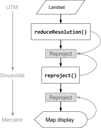
איור 3. תרשים זרימה של הפעולות כשפונים ל-reduceResolution() בתמונה קלט לפני reproject(). הקווים המעוקלים מציינים את זרימת המידע להקרנה מחדש: באופן ספציפי, את שיטת ההקרנה, הסולם והצבירה של הפיקסלים של הפלט.

הערה: מתבצעת הקרנה מחדש שנייה (באופן משתמע) כדי להציג את הנתונים במפה של Code Editor. בודקים את התוצאות באופן חזותי ומתבוננים בהתאמה בין הפיקסלים משכבת MODIS לבין נתוני כיסוי היער שהופרויקטטו מחדש בקנה המידה והתצוגה של MODIS. בדרך כלל לא תצטרכו להשתמש ב-reproject() באופן מפורש ב-Earth Engine.

משקלים של פיקסלים עבור ReduceResolution

המשקלים של הפיקסלים שמשמשים בתהליך הצבירה של reduceResolution() מבוססים על החפיפה בין הפיקסלים הקטנים שמצטברים לבין הפיקסלים הגדולים שצוינו על ידי הקרנת הפלט. הדוגמה הזו מופיעה באיור 4.

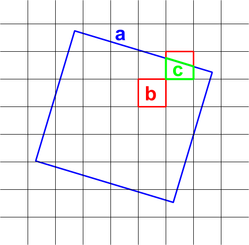
איור 4. פיקסלים של קלט (שחור) ופיקסל של פלט (כחול) עבור reduceResolution().

ברירת המחדל היא שמשקל הפיקסלים בקלט מחושבים כחלק משטח הפיקסלים של הפלט שמכוסה על ידי פיקסל הקלט. בתרשים, שטח הפיקסל של הפלט הוא a, המשקל של פיקסל הקלט עם שטח החיתוך b מחושב כ-b/a והמשקל של פיקסל הקלט עם שטח החיתוך c מחושב כ-c/a. ההתנהגות הזו עלולה לגרום לתוצאות לא צפויות כשמשתמשים במצמצם שאינו המצמצם של הממוצע. לדוגמה, כדי לחשב את שטח היער לכל פיקסל, משתמשים במצמצם הממוצע כדי לחשב את החלק של הפיקסל המכוסה, ואז מכפילים בשטח (במקום לחשב את השטחים בפיקסלים הקטנים יותר ואז להוסיף אותם באמצעות מצמצם הסכום):

Code Editor‏ (JavaScript)

// Compute forest area per MODIS pixel.
var forestArea = forest.gt(0)
    // Force the next reprojection to aggregate instead of resampling.
    .reduceResolution({
      reducer: ee.Reducer.mean(),
      maxPixels: 1024
    })
    // The reduce resolution returns the fraction of the MODIS pixel
    // that's covered by 30 meter forest pixels.  Convert to area
    // after the reduceResolution() call.
    .multiply(ee.Image.pixelArea())
    // Request the data at the scale and projection of the MODIS image.
    .reproject({
      crs: modisProjection
    });
Map.addLayer(forestArea, {max: 500 * 500}, 'forested area at MODIS scale');

הגדרת Python

בדף סביבת Python מפורט מידע על Python API ועל השימוש ב-geemap לפיתוח אינטראקטיבי.

import ee
import geemap.core as geemap

Colab (Python)

# Compute forest area per MODIS pixel.
forest_area = (
    forest.gt(0)
    # Force the next reprojection to aggregate instead of resampling.
    .reduceResolution(reducer=ee.Reducer.mean(), maxPixels=1024)
    # The reduce resolution returns the fraction of the MODIS pixel
    # that's covered by 30 meter forest pixels.  Convert to area
    # after the reduceResolution() call.
    .multiply(ee.Image.pixelArea())
    # Request the data at the scale and projection of the MODIS image.
    .reproject(crs=modis_projection)
)
m.add_layer(forest_area, {'max': 500 * 500}, 'forested area at MODIS scale')
m