Warstwa danych dotycząca intensywności zmian występowania wody dostarcza informacji o tym, jak wody powierzchniowe zmieniły się w okresach 1984–1999 i 2000–2015. Warstwa uśrednia zmianę w przypadku homologicznych par miesięcy z obu epok. Więcej informacji o tej warstwie znajdziesz w przewodniku użytkownika danych (wersja 2) .
W tej części samouczka:
- dodawać warstwę mapy ze stylem do wizualizacji intensywności zmian występowania wody,
- podsumowywać intensywność zmian w określonym obszarze zainteresowania za pomocą histogramu;
Wizualizacja
Podobnie jak w przypadku warstwy występowania wody, zaczniemy od dodania do mapy podstawowej wizualizacji intensywności zmiany występowania, a następnie będziemy ją ulepszać. Intensywność zmiany występowania jest podawana na 2 sposoby: jako wartość bezwzględna i jako wartość znormalizowana. W tym samouczku będziemy używać wartości bezwzględnych. Zacznij od wybrania warstwy intensywności zmiany bezwzględnej liczby wystąpień na obrazie GSW:
Edytor kodu (JavaScript)
var change = gsw.select("change_abs");
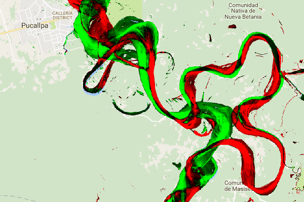
W sekcji stałych w kodzie dodaj instrukcję, która utworzy nową zmienną określającą stylizację warstwy. Ten styl pokazuje obszary, w których występowanie wód powierzchniowych zmniejszyło się lub zwiększyło, odpowiednio w kolorze czerwonym lub zielonym. Obszary, na których występowanie wód powierzchniowych jest stosunkowo niezmienione, są oznaczone na czarno.
Edytor kodu (JavaScript)
var VIS_CHANGE = {
    min:-50,
    max:50,
    palette: ['red', 'black', 'limegreen']
};
Na końcu sekcji kodu Map Layers (Warstwy mapy) dodaj instrukcję, która doda nową warstwę do mapy.
Edytor kodu (JavaScript)
Map.setCenter(-74.4557, -8.4289, 11);  // Ucayali River, Peru
Map.addLayer({
  eeObject: change,
  visParams: VIS_CHANGE,
  name: 'occurrence change intensity'
});
Podsumowywanie zmian w obszarze zainteresowań
W tej sekcji podsumujemy zakres zmian w określonym regionie, który Cię interesuje. Aby określić obszar zainteresowania, kliknij narzędzie do rysowania wielokątów, które jest jednym z narzędzi do rysowania kształtów. Spowoduje to utworzenie nowej warstwy importu geometrii, która domyślnie ma nazwę „geometry”. Aby zmienić nazwę, kliknij ikonę koła zębatego po prawej stronie nazwy warstwy. (Aby wyświetlić nazwę warstwy, może być konieczne umieszczenie na niej kursora).
Zmień nazwę warstwy na roi (dla regionu zainteresowania). Następnie możemy kliknąć serię punktów na mapie, aby zdefiniować wielokątny region zainteresowania.
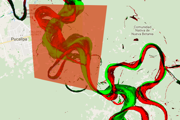
Teraz, gdy nasz obszar zainteresowania jest zdefiniowany i przechowywany w zmiennej, możemy go użyć do obliczenia histogramu intensywności zmian dla tego obszaru. Dodaj ten kod do sekcji Obliczenia w skrypcie.
Edytor kodu (JavaScript)
// Calculate a change intensity for the region of interest.
var histogram = change.reduceRegion({
  reducer: ee.Reducer.histogram(),
  geometry: roi,
  scale: 30,
  bestEffort: true,
});
print(histogram);
Pierwsza instrukcja oblicza histogram wartości intensywności zmiany występowania w obszarze zainteresowania, próbkowany w skali 30 m. Druga instrukcja wyświetla wynikowy obiekt na karcie Konsola w edytorze kodu. Możesz rozwinąć drzewo obiektów, aby wyświetlić wartości przedziałów histogramu. Dane liczbowe są dostępne, ale istnieją lepsze sposoby wizualizacji wyników.

Aby to poprawić, możemy zamiast tego wygenerować histogram. Zastąp instrukcję, która definiuje obiekt histogramu, tymi instrukcjami:
Edytor kodu (JavaScript)
// Generate a histogram object and print it to the console tab.
var histogram = ui.Chart.image.histogram({
  image: change,
  region: roi,
  scale: 30,
  minBucketWidth: 10
});
histogram.setOptions({
  title: 'Histogram of surface water change intensity.'
});
Te instrukcje tworzą obiekt wykresu histogramu, który zastępuje drzewo obiektów histogramu na karcie Konsola wykresem. Metoda wykresu zawiera kilka argumentów, w tym scale, który określa skalę przestrzenną w metrach, w której próbkowany jest interesujący nas region, oraz minBucketWidth, który służy do kontrolowania szerokości zasobników histogramu.
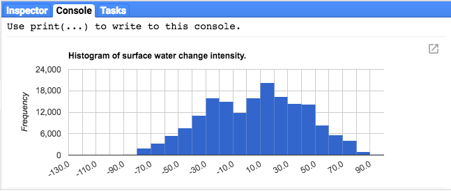
Wartości wykresu możesz sprawdzać interaktywnie, umieszczając kursor nad słupkami histogramu.
Skrypt końcowy
Cały skrypt tej sekcji znajdziesz poniżej. Zwróć uwagę, że skrypt zawiera instrukcje definiujące geometrię wielokąta (roi), która jest porównywalna z geometrią utworzoną za pomocą narzędzi do geometrii w edytorze kodu.
Edytor kodu (JavaScript)
//////////////////////////////////////////////////////////////
// Asset List
//////////////////////////////////////////////////////////////

var gsw = ee.Image('JRC/GSW1_0/GlobalSurfaceWater');
var occurrence = gsw.select('occurrence');
var change = gsw.select("change_abs");
var roi = /* color: 0B4A8B */ee.Geometry.Polygon(
        [[[-74.17213, -8.65569],
          [-74.17419, -8.39222],
          [-74.38362, -8.36980],
          [-74.43031, -8.61293]]]);

//////////////////////////////////////////////////////////////
// Constants
//////////////////////////////////////////////////////////////

var VIS_OCCURRENCE = {
    min:0,
    max:100,
    palette: ['red', 'blue']
};
var VIS_CHANGE = {
    min:-50,
    max:50,
    palette: ['red', 'black', 'limegreen']
};
var VIS_WATER_MASK = {
  palette: ['white', 'black']
};

//////////////////////////////////////////////////////////////
// Calculations
//////////////////////////////////////////////////////////////

// Create a water mask layer, and set the image mask so that non-water areas are transparent.
var water_mask = occurrence.gt(90).mask(1);

// Generate a histogram object and print it to the console tab.
var histogram = ui.Chart.image.histogram({
  image: change,
  region: roi,
  scale: 30,
  minBucketWidth: 10
});
histogram.setOptions({
  title: 'Histogram of surface water change intensity.'
});
print(histogram);

//////////////////////////////////////////////////////////////
// Initialize Map Location
//////////////////////////////////////////////////////////////

// Uncomment one of the following statements to center the map on
// a particular location.
// Map.setCenter(-90.162, 29.8597, 10);   // New Orleans, USA
// Map.setCenter(-114.9774, 31.9254, 10); // Mouth of the Colorado River, Mexico
// Map.setCenter(-111.1871, 37.0963, 11); // Lake Powell, USA
// Map.setCenter(149.412, -35.0789, 11);  // Lake George, Australia
// Map.setCenter(105.26, 11.2134, 9);     // Mekong River Basin, SouthEast Asia
// Map.setCenter(90.6743, 22.7382, 10);   // Meghna River, Bangladesh
// Map.setCenter(81.2714, 16.5079, 11);   // Godavari River Basin Irrigation Project, India
// Map.setCenter(14.7035, 52.0985, 12);   // River Oder, Germany & Poland
// Map.setCenter(-59.1696, -33.8111, 9);  // Buenos Aires, Argentina\
Map.setCenter(-74.4557, -8.4289, 11);  // Ucayali River, Peru

//////////////////////////////////////////////////////////////
// Map Layers
//////////////////////////////////////////////////////////////

Map.addLayer({
  eeObject: water_mask,
  visParams: VIS_WATER_MASK,
  name: '90% occurrence water mask',
  shown: false
});
Map.addLayer({
  eeObject: occurrence.updateMask(occurrence.divide(100)),
  name: "Water Occurrence (1984-2015)",
  visParams: VIS_OCCURRENCE,
  shown: false
});
Map.addLayer({
  eeObject: change,
  visParams: VIS_CHANGE,
  name: 'occurrence change intensity'
});
W następnej sekcji dowiesz się więcej o tym, jak zmieniała się woda na przestrzeni czasu, pracując z warstwą przejścia klasy wody.