

构成 ImageCollection 的图像可以可视化为动画或一系列缩略图(称为“幻灯影片”)。这些方法可让您快速评估 ImageCollection 的内容,并提供见证时空变化的有效媒介(图 1)。
getVideoThumbURL()生成动画图片系列getFilmstripThumbURL()生成一系列缩略图
以下部分介绍了如何准备 ImageCollection 以进行可视化,提供了每种集合可视化方法的示例代码,并介绍了多种高级动画技术。
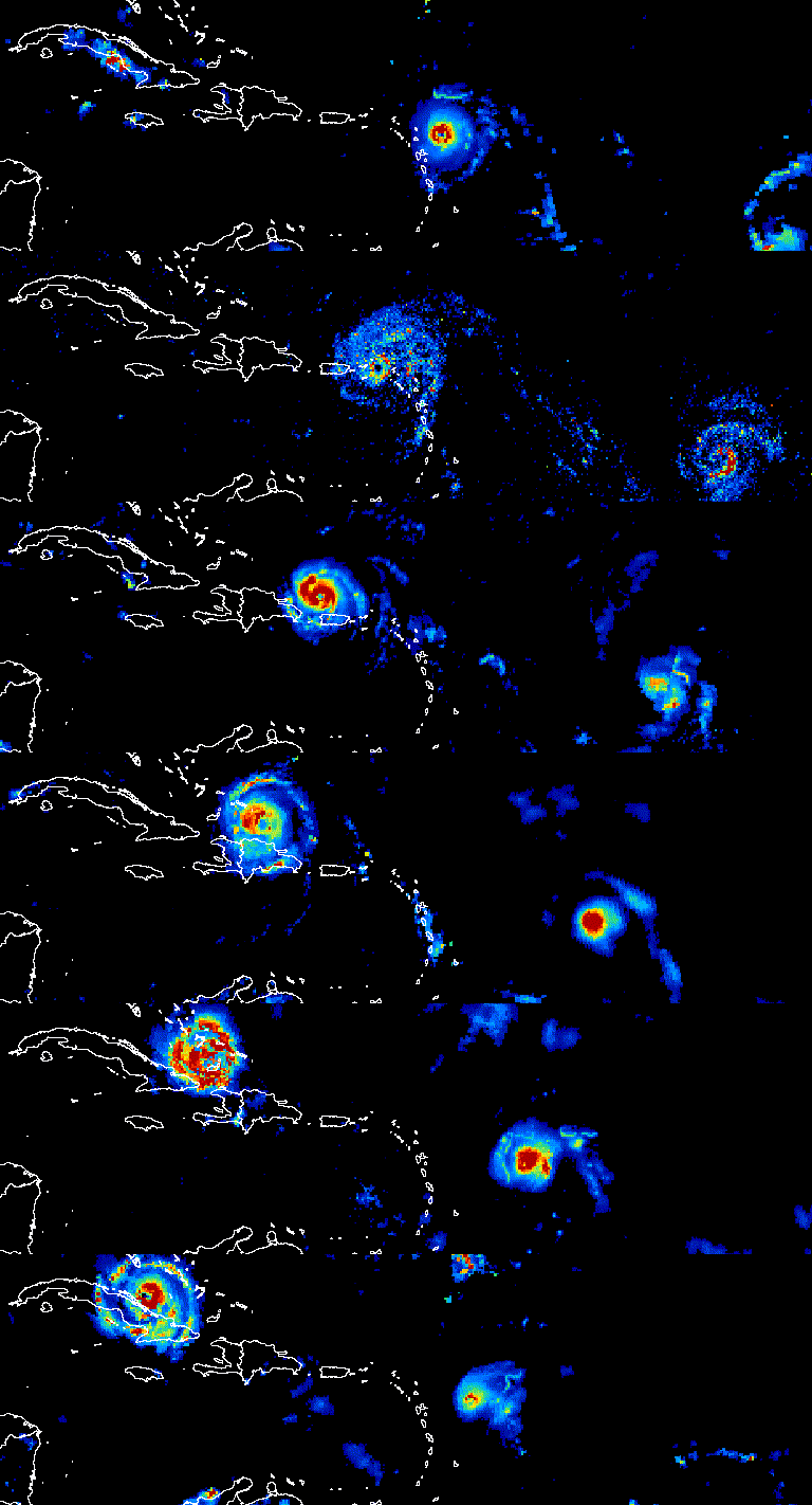
图 1. 动画显示了 2017 年 9 月大西洋飓风的三天演变过程。
收集准备
对集合中的图片进行过滤、合成、排序和样式设置,以便仅显示感兴趣的图片或突出显示某种现象。任何 ImageCollection 都可以作为可视化函数的输入,但如果能考虑到年际和年内日期范围、观测间隔、区域范围、质量和代表性,则可以获得更好的结果。
过滤条件
过滤图片集合,使其仅包含支持可视化目的的相关数据。考虑特定于给定数据集的日期、空间范围、质量和其他属性。
例如,按以下条件过滤 Sentinel-2 地表反射率集合:
单个日期范围
代码编辑器 (JavaScript)
var s2col = ee.ImageCollection('COPERNICUS/S2_SR_HARMONIZED')
  .filterDate('2018-01-01', '2019-01-01');
一个连续的日期范围,
代码编辑器 (JavaScript)
var s2col = ee.ImageCollection('COPERNICUS/S2_SR_HARMONIZED')
  .filter(ee.Filter.calendarRange(171, 242, 'day_of_year'));
查看感兴趣的地区
代码编辑器 (JavaScript)
var s2col = ee.ImageCollection('COPERNICUS/S2_SR_HARMONIZED')
  .filterBounds(ee.Geometry.Point(-122.1, 37.2));
或图片属性。
代码编辑器 (JavaScript)
var s2col = ee.ImageCollection('COPERNICUS/S2_SR_HARMONIZED')
  .filter(ee.Filter.lt('CLOUDY_PIXEL_PERCENTAGE', 50));
串联多个滤镜。
代码编辑器 (JavaScript)
var s2col = ee.ImageCollection('COPERNICUS/S2_SR_HARMONIZED')
  .filterDate('2018-01-01', '2019-01-01')
  .filterBounds(ee.Geometry.Point(-122.1, 37.2))
  .filter('CLOUDY_PIXEL_PERCENTAGE < 50');
复合
合成年内和年际日期范围,以减少集合中的图片数量并提高质量。例如,假设您要创建非洲年度 NDVI 的可视化图表。一种方法是简单地过滤 MODIS 16 天 NDVI 集合,以包含 2018 年的所有观测数据。
代码编辑器 (JavaScript)
var ndviCol = ee.ImageCollection('MODIS/061/MOD13A2')
  .filterDate('2018-01-01', '2019-01-01')
  .select('NDVI');
通过过滤和缩减进行年际合成
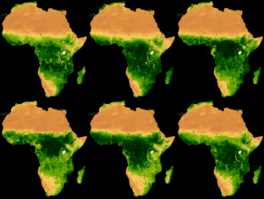
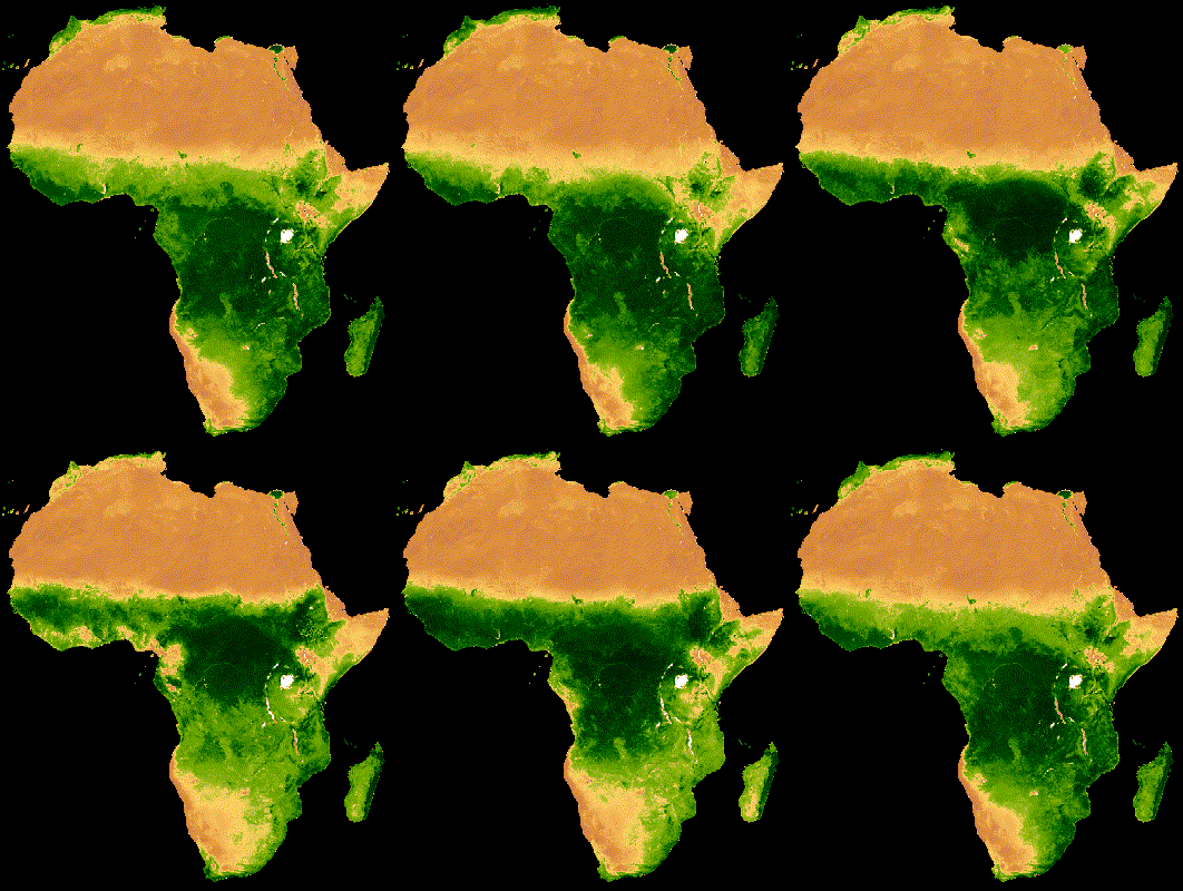
上述集合的可视化结果显示,在云层较厚的森林区域存在大量噪声(图 2a)。通过在 MODIS 集合中按所有年份的中位数减少连续日期范围,可以实现更好的表示。
代码编辑器 (JavaScript)
// Make a day-of-year sequence from 1 to 365 with a 16-day step.
var doyList = ee.List.sequence(1, 365, 16);

// Import a MODIS NDVI collection.
var ndviCol = ee.ImageCollection('MODIS/061/MOD13A2').select('NDVI');

// Map over the list of days to build a list of image composites.
var ndviCompList = doyList.map(function(startDoy) {
  // Ensure that startDoy is a number.
  startDoy = ee.Number(startDoy);

  // Filter images by date range; starting with the current startDate and
  // ending 15 days later. Reduce the resulting image collection by median.
  return ndviCol
    .filter(ee.Filter.calendarRange(startDoy, startDoy.add(15), 'day_of_year'))
    .reduce(ee.Reducer.median());
});

// Convert the image List to an ImageCollection.
var ndviCompCol = ee.ImageCollection.fromImages(ndviCompList);
此集合生成的动画噪点较少,因为每张图片都代表 20 多年数据中 16 天 NDVI 合成图像的中位数(图 1b)。如需详细了解此动画,请参阅此教程。
 |
 |
|---|---|
| 图 2a. 未进行年际合成的年度 NDVI。 | 图 2b. 采用年际合成的年度 NDVI。 |
通过过滤和缩减进行年内合成
上一个示例应用了跨年度合成。合成一系列年内观测数据也很有帮助。例如,Landsat 数据是每个传感器每 16 天收集一次给定场景的数据,但通常部分图像会被云层遮挡。遮盖云层并合成同一季节的多张图片,可以生成更清晰的无云图像。请考虑以下示例:使用 1985 年至 2011 年间每年 7 月和 8 月的 Landsat 5 影像,通过中位数方法进行合成。
代码编辑器 (JavaScript)
// Assemble a collection of Landsat surface reflectance images for a given
// region and day-of-year range.
var lsCol = ee.ImageCollection('LANDSAT/LT05/C02/T1_L2')
  .filterBounds(ee.Geometry.Point(-122.9, 43.6))
  .filter(ee.Filter.dayOfYear(182, 243))
  // Add the observation year as a property to each image.
  .map(function(img) {
    return img.set('year', ee.Image(img).date().get('year'));
  });


// Define a function to scale the data and mask unwanted pixels.
function maskL457sr(image) {
  // Bit 0 - Fill
  // Bit 1 - Dilated Cloud
  // Bit 2 - Unused
  // Bit 3 - Cloud
  // Bit 4 - Cloud Shadow
  var qaMask = image.select('QA_PIXEL').bitwiseAnd(parseInt('11111', 2)).eq(0);
  var saturationMask = image.select('QA_RADSAT').eq(0);

  // Apply the scaling factors to the appropriate bands.
  var opticalBands = image.select('SR_B.').multiply(0.0000275).add(-0.2);
  var thermalBand = image.select('ST_B6').multiply(0.00341802).add(149.0);

  // Replace the original bands with the scaled ones and apply the masks.
  return image.addBands(opticalBands, null, true)
      .addBands(thermalBand, null, true)
      .updateMask(qaMask)
      .updateMask(saturationMask);
}

// Define a list of unique observation years from the image collection.
var years = ee.List(lsCol.aggregate_array('year')).distinct().sort();

// Map over the list of years to build a list of annual image composites.
var lsCompList = years.map(function(year) {
  return lsCol
    // Filter image collection by year.
    .filterMetadata('year', 'equals', year)
    // Apply cloud mask.
    .map(maskL457sr)
    // Reduce image collection by median.
    .reduce(ee.Reducer.median())
    // Set composite year as an image property.
    .set('year', year);
});

// Convert the image List to an ImageCollection.
var lsCompCol = ee.ImageCollection.fromImages(lsCompList);
通过联接和缩减实现的年内合成
请注意,前两种合成方法会映射到 List 的天数和年份,以逐步定义要过滤和合成的新日期。
应用联接是实现此操作的另一种方法。在以下代码段中,定义了一个唯一的年份集合,然后应用 saveAll 联接来识别与给定年份对应的所有图片。属于给定年份的图片会分组到一个 List 对象中,该对象会作为不同年份集合中相应年份代表的属性进行存储。年度合成图像是通过在映射到不同年份集合的函数中缩减这些列表定义的 ImageCollections 生成的。
代码编辑器 (JavaScript)
// Assemble a collection of Landsat surface reflectance images for a given
// region and day-of-year range.
var lsCol = ee.ImageCollection('LANDSAT/LT05/C02/T1_L2')
  .filterBounds(ee.Geometry.Point(-122.9, 43.6))
  .filter(ee.Filter.dayOfYear(182, 243))
  // Add the observation year as a property to each image.
  .map(function(img) {
    return img.set('year', ee.Image(img).date().get('year'));
  });

// Make a distinct year collection; one image representative per year.
var distinctYears = lsCol.distinct('year').sort('year');

// Define a join filter; one-to-many join on ‘year’ property.
var filter = ee.Filter.equals({leftField: 'year', rightField: 'year'});

// Define a join.
var join = ee.Join.saveAll('year_match');

// Apply the join; results in 'year_match' property being added to each distinct
// year representative image. The list includes all images in the collection
// belonging to the respective year.
var joinCol = join.apply(distinctYears, lsCol, filter);

// Define a function to scale the data and mask unwanted pixels.
function maskL457sr(image) {
  // Bit 0 - Fill
  // Bit 1 - Dilated Cloud
  // Bit 2 - Unused
  // Bit 3 - Cloud
  // Bit 4 - Cloud Shadow
  var qaMask = image.select('QA_PIXEL').bitwiseAnd(parseInt('11111', 2)).eq(0);
  var saturationMask = image.select('QA_RADSAT').eq(0);

  // Apply the scaling factors to the appropriate bands.
  var opticalBands = image.select('SR_B.').multiply(0.0000275).add(-0.2);
  var thermalBand = image.select('ST_B6').multiply(0.00341802).add(149.0);

  // Replace the original bands with the scaled ones and apply the masks.
  return image.addBands(opticalBands, null, true)
      .addBands(thermalBand, null, true)
      .updateMask(qaMask)
      .updateMask(saturationMask);
}

// Map over the distinct years collection to build a list of annual image
// composites.
var lsCompList = joinCol.map(function(img) {
  // Get the list of images belonging to the given year.
  return ee.ImageCollection.fromImages(img.get('year_match'))
    // Apply cloud mask.
    .map(maskL457sr)
    // Reduce image collection by median.
    .reduce(ee.Reducer.median())
    // Set composite year as an image property.
    .copyProperties(img, ['year']);
});

// Convert the image List to an ImageCollection.
var lsCompCol = ee.ImageCollection(lsCompList);
通过联接和缩减操作实现当天合成
合成的另一个应用场景是创建空间连续的图像拼接。假设您感兴趣的区域跨越同一路径中的两个 Landsat 行,而您的目标是显示 2017 年和 2018 年每个 Landsat 8 轨道的两张图片的拼接图像。在这里,按路径和行过滤集合后,使用联接操作来拼接来自同一轨道的 Landsat 图像(由获取日期定义)。
代码编辑器 (JavaScript)
var lsCol = ee.ImageCollection('LANDSAT/LC08/C02/T1_L2')
  .filterDate('2017-01-01', '2019-01-01')
  .filter('WRS_PATH == 38 && (WRS_ROW == 28 || WRS_ROW == 29)')
  .map(function(img) {
    var date = img.date().format('yyyy-MM-dd');
    return img.set('date', date);
  });

var distinctDates = lsCol.distinct('date').sort('date');
var filter = ee.Filter.equals({leftField: 'date', rightField: 'date'});
var join = ee.Join.saveAll('date_match');
var joinCol = join.apply(distinctDates, lsCol, filter);

var lsColMos = ee.ImageCollection(joinCol.map(function(col) {
  return ee.ImageCollection.fromImages(col.get('date_match')).mosaic();
}));
排序
按时间对集合进行排序,以确保正确的时间顺序,或按您选择的属性进行排序。默认情况下,可视化框架系列按集合的自然顺序排序。您可以使用 sort 集合方法更改序列的排列方式,从而选择 Image 属性以升序或降序排序。例如,如需按观察时间排序,请使用无处不在的 system:time_start 属性。
代码编辑器 (JavaScript)
var s2col = ee.ImageCollection('COPERNICUS/S2_SR_HARMONIZED')
  .filterBounds(ee.Geometry.Point(-122.1, 37.2))
  .sort('system:time_start');
或者,也可以按云量递增的顺序排列,如 Sentinel-2 图像。
代码编辑器 (JavaScript)
var s2col = ee.ImageCollection('COPERNICUS/S2_SR_HARMONIZED')
  .filterBounds(ee.Geometry.Point(-122.1, 37.2))
  .sort('CLOUDY_PIXEL_PERCENTAGE');
顺序也可以由派生属性定义,例如区域平均 NDVI。 在这里,区域 NDVI 作为属性添加到映射函数中的每个图像,然后对新属性进行排序。
代码编辑器 (JavaScript)
// Define an area of interest geometry.
var aoi = ee.Geometry.Point(-122.1, 37.2).buffer(1e4);

// Filter MODIS NDVI image collection by a date range.
var ndviCol = ee.ImageCollection('MODIS/061/MOD13A1')
  .filterDate('2018-01-01', '2019-01-01')
  .select('NDVI')
  // Map over the image collection to calculate regional mean NDVI and add
  // the result to each image as a property.
  .map(function(img) {
    var meanNdvi = img.reduceRegion({
      reducer: ee.Reducer.mean(), geometry: aoi, scale: 500});
    return img.set('meanNdvi', meanNdvi.get('NDVI'));
  })
  // Sort the collection by descending regional mean NDVI.
  .sort('meanNdvi', false);
图片可视化
图像可视化会将数字转换为颜色。您可以通过以下三种方式来控制在集合可视化方法中如何将图片数据表示为颜色:
- 直接向
getVideoThumbURL和getFilmstripThumbURL提供可视化参数。 - 在应用
getVideoThumbURL和getFilmstripThumbURL之前,先将visualize图片方法映射到图片集合。 - 在应用
getVideoThumbURL和getFilmstripThumbURL之前,先将sldStyle图片方法映射到图片集合。如需了解详情,请参阅样式化图层描述符。
本指南中的示例使用选项 1 和 2,其中通过将多波段图像的三个图像波段映射到颜色通道红色、绿色和蓝色或沿调色板线性分级单个波段的值来实现可视化。可视化参数包括:
| 参数 | 说明 | 类型 |
|---|---|---|
| 频段 | 要映射到 RGB 的三个波段名称的英文逗号分隔列表 | list |
| 分钟 | 要映射到 0 的值 | 数字或包含三个数字的列表(每个波段一个数字) |
| 最大值 | 要映射到 255 的值 | 数字或包含三个数字的列表(每个波段一个数字) |
| gain | 每个像素值要乘以的值 | 数字或包含三个数字的列表(每个波段一个数字) |
| 偏见 | 要添加到每个 DN 的值 | 数字或包含三个数字的列表(每个波段一个数字) |
| gamma | 伽马校正系数 | 数字或包含三个数字的列表(每个波段一个数字) |
| palette | CSS 样式颜色字符串列表(仅限单波段图片) | 以英文逗号分隔的十六进制字符串列表 |
| 不透明度 | 图层的不透明度(0.0 表示完全透明,1.0 表示完全不透明) | 数值 |
使用 bands 参数选择要直观呈现的波段。提供一个或三个波段名称的列表。对于多波段图片,系统会默认选择前三个波段。波段名称顺序决定了颜色分配;列出的第一、第二和第三个波段分别映射到红色、绿色和蓝色。
在直观呈现图片时,数据范围缩放是一个重要的考虑因素。默认情况下,介于 0 和 1(含)之间的浮点数据值会缩放到 0 到 255(含)之间。此范围之外的值会被强制设为 0 和 255,具体取决于它们是小于 0 还是大于 1。对于整数数据,其类型定义的完整容量会缩放到 0 到 255 之间(例如,有符号 16 位数据的范围为 -32,768 到 32,767,默认情况下会缩放到 [0, 255])。接受默认值通常会导致可视化图表中的图像特征之间几乎没有对比度。使用 min 和 max 可提高对比度并突出显示特定数据范围。一个很好的经验法则是,将 min 和 max 设置为代表感兴趣区域内数据的第 2 个和第 98 个百分位数的值。请参阅以下示例,了解如何为数字高程模型计算这些值。
代码编辑器 (JavaScript)
// Import NASADEM global elevation model.
var demImg = ee.Image('NASA/NASADEM_HGT/001').select('elevation');

// Define a rectangular area of interest.
var aoi = ee.Geometry.Polygon(
  [[
    [-103.84153083119054, 49.083004219142886],
    [-103.84153083119054, 25.06838270664608],
    [-85.64817145619054, 25.06838270664608],
    [-85.64817145619054, 49.083004219142886]
  ]],
  null, false);

// Calculate the 2nd and 98th percentile elevation values from rescaled (to
// 500m) pixels intersecting the area of interest. A Dictionary is returned.
var percentClip = demImg.reduceRegion({
  reducer: ee.Reducer.percentile([2, 98]),
  geometry: aoi,
  scale: 500,
  maxPixels: 3e7
});

// Print the regional 2nd and 98th percentile elevation values. Get the
// dictionary keys and use them to get the values for each percentile summary.
var keys = percentClip.keys();
print('Set vis min to:', ee.Number(percentClip.get(keys.get(0))).round());
print('Set vis max to:', ee.Number(percentClip.get(keys.get(1))).round());
palette 参数定义了用于表示 8 位可视化图片的颜色。它仅适用于单波段表示法;如果指定多波段图片,则会导致错误。如果数据是单波段,或者您想直观呈现多波段图像中的单个波段,请将 forceRgbOutput 参数设置为 true(如果提供了 palette 参数,则无需设置)。使用 min 和 max 参数定义要在 0 到 255 之间线性缩放的值范围。
以下示例展示了如何将可视化函数映射到单波段图像集合。导入 MODIS NDVI 集合,设置 visualization 方法的可视化参数,并将一个将值转换为 RGB 图像表示形式的函数映射到 NDVI 集合。
代码编辑器 (JavaScript)
// Filter MODIS NDVI image collection by a date range.
var ndviCol = ee.ImageCollection('MODIS/061/MOD13A1')
  .filterDate('2018-01-01', '2019-01-01')
  .select('NDVI');

// Define visualization arguments.
var visArgs = {
  min: 0,
  max: 9000,
  palette: [
    'FFFFFF', 'CE7E45', 'DF923D', 'F1B555', 'FCD163', '99B718', '74A901',
    '66A000', '529400', '3E8601', '207401', '056201', '004C00', '023B01',
    '012E01', '011D01', '011301'
  ]
};

// Define a function to convert an image to an RGB visualization image and copy
// properties from the original image to the RGB image.
var visFun = function(img) {
  return img.visualize(visArgs).copyProperties(img, img.propertyNames());
};

// Map over the image collection to convert each image to an RGB visualization
// using the previously defined visualization function.
var ndviColVis = ndviCol.map(visFun);
以下是针对多波段图片集合映射可视化函数的示例:
代码编辑器 (JavaScript)
// Assemble a collection of Sentinel-2 surface reflectance images for a given
// region and date range.
var s2col = ee.ImageCollection('COPERNICUS/S2_SR_HARMONIZED')
  .filterBounds(ee.Geometry.Point(-96.9037, 48.0395))
  .filterDate('2019-06-01', '2019-10-01');

// Define visualization arguments.
var visArgs = {bands: ['B11', 'B8', 'B3'], min: 300, max: 3500};

// Define a function to convert an image to an RGB visualization image and copy
// properties from the original image to the RGB image.
var visFun = function(img) {
  return img.visualize(visArgs).copyProperties(img, img.propertyNames());
};

// Map over the image collection to convert each image to an RGB visualization
// using the previously defined visualization function.
var s2colVis = s2col.map(visFun);
在这种情况下,由于提供了三个波段,因此无需提供调色板参数,这些波段定义了每个 RGB 层的强度。请注意,这两个示例都使用 min 和 max 参数来控制将哪些值拉伸到 8 位 RGB 数据的极限。
视频缩略图
getVideoThumbURL() 函数会根据 ImageCollection 中的所有图片生成动画,其中每张图片代表一帧。制作动画的一般工作流程如下:
- 定义一个
Geometry,其边界决定了动画的区域范围。 - 定义
ImageCollection。 - 考虑图片可视化:将图片可视化函数映射到集合,或将图片可视化参数添加到动画参数集中。
- 定义动画参数并调用
getVideoThumbURL方法。
getVideoThumbURL 的结果是一个网址。将网址输出到控制台,然后点击该网址,让 Earth Engine 服务器在新的浏览器标签页中实时生成动画。或者,您也可以在集合及其对应的动画参数上调用 ui.Thumbnail 函数,在代码编辑器控制台中查看动画。渲染后,右键点击动画并从其上下文菜单中选择适当的选项,即可下载动画。
以下示例展示了如何生成描绘 24 小时内全球温度的动画。请注意,此示例包含可视化参数和动画参数,而不是先在 ImageCollection 上映射可视化函数。运行此脚本后,代码编辑器控制台中应会显示类似于图 3 的动画。
代码编辑器 (JavaScript)
// Define an area of interest geometry with a global non-polar extent.
var aoi = ee.Geometry.Polygon(
  [[[-179.0, 78.0], [-179.0, -58.0], [179.0, -58.0], [179.0, 78.0]]], null,
  false);

// Import hourly predicted temperature image collection for northern winter
// solstice. Note that predictions extend for 384 hours; limit the collection
// to the first 24 hours.
var tempCol = ee.ImageCollection('NOAA/GFS0P25')
  .filterDate('2018-12-22', '2018-12-23')
  .limit(24)
  .select('temperature_2m_above_ground');

// Define arguments for animation function parameters.
var videoArgs = {
  dimensions: 768,
  region: aoi,
  framesPerSecond: 7,
  crs: 'EPSG:3857',
  min: -40.0,
  max: 35.0,
  palette: ['blue', 'purple', 'cyan', 'green', 'yellow', 'red']
};

// Print the animation to the console as a ui.Thumbnail using the above defined
// arguments. Note that ui.Thumbnail produces an animation when the first input
// is an ee.ImageCollection instead of an ee.Image.
print(ui.Thumbnail(tempCol, videoArgs));

// Alternatively, print a URL that will produce the animation when accessed.
print(tempCol.getVideoThumbURL(videoArgs));
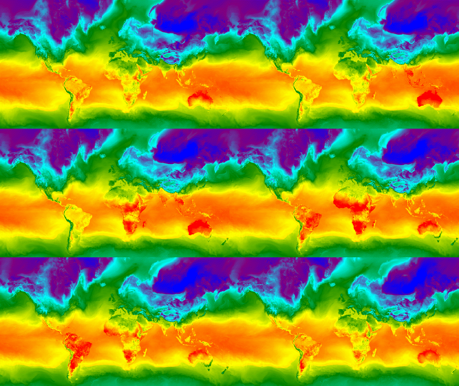
图 3. 北半球冬至期间的每小时地表温度,以 GIF 动画图片表示。
视频片段
getFilmstripThumbUrl 函数会生成一个静态图片,表示将 ImageCollection 中的所有图片串联成一个南北系列。幻灯影片帧的顺序遵循集合的自然顺序。
getFilmstripThumbUrl 的结果是一个网址。将网址输出到控制台,然后点击该网址,让 Earth Engine 服务器在新的浏览器标签页中实时生成图片。渲染后,您可以通过右键点击图片并从其上下文菜单中选择适当的选项来下载图片。
以下代码段使用与上述视频缩略图示例相同的集合。运行此脚本后,代码编辑器控制台中应会显示类似于图 4 的幻灯影片。
代码编辑器 (JavaScript)
// Define an area of interest geometry with a global non-polar extent.
var aoi = ee.Geometry.Polygon(
  [[[-179.0, 78.0], [-179.0, -58.0], [179.0, -58.0], [179.0, 78.0]]], null,
  false);

// Import hourly predicted temperature image collection for northern winter
// solstice. Note that predictions extend for 384 hours; limit the collection
// to the first 24 hours.
var tempCol = ee.ImageCollection('NOAA/GFS0P25')
  .filterDate('2018-12-22', '2018-12-23')
  .limit(24)
  .select('temperature_2m_above_ground');

// Define arguments for the getFilmstripThumbURL function parameters.
var filmArgs = {
  dimensions: 128,
  region: aoi,
  crs: 'EPSG:3857',
  min: -40.0,
  max: 35.0,
  palette: ['blue', 'purple', 'cyan', 'green', 'yellow', 'red']
};

// Print a URL that will produce the filmstrip when accessed.
print(tempCol.getFilmstripThumbURL(filmArgs));

图 4. 北半球冬至日每小时地表温度,以幻灯影片 PNG 图片表示。请注意,幻灯影片已分为四个部分进行显示;getFilmstripThumbURL 的结果是南北方向拼接的一系列集合图片。
高级技术
以下部分介绍了如何使用裁剪、不透明度和图层合成功能,通过添加多边形边框、突出显示感兴趣的区域以及比较集合中的图片来增强可视化效果。
请注意,本部分中的以下所有示例都使用此处定义的相同基本 ImageCollection:
代码编辑器 (JavaScript)
// Import hourly predicted temperature image collection for northern winter
// solstice. Note that predictions extend for 384 hours; limit the collection
// to the first 24 hours.
var tempCol = ee.ImageCollection('NOAA/GFS0P25')
  .filterDate('2018-12-22', '2018-12-23')
  .limit(24)
  .select('temperature_2m_above_ground');

// Define visualization arguments to control the stretch and color gradient
// of the data.
var visArgs = {
  min: -40.0,
  max: 35.0,
  palette: ['blue', 'purple', 'cyan', 'green', 'yellow', 'red']
};

// Convert each image to an RGB visualization image by mapping the visualize
// function over the image collection using the arguments defined previously.
var tempColVis = tempCol.map(function(img) {
  return img.visualize(visArgs);
});

// Import country features and filter to South American countries.
var southAmCol = ee.FeatureCollection('USDOS/LSIB_SIMPLE/2017')
  .filterMetadata('wld_rgn', 'equals', 'South America');

// Define animation region (South America with buffer).
var southAmAoi = ee.Geometry.Rectangle({
  coords: [-103.6, -58.8, -18.4, 17.4], geodesic: false});
叠加层
您可以使用 blend Image 方法叠加多张图片,其中两张图片中重叠的像素会根据其遮罩(不透明度)进行混合。
矢量叠加层
向图片添加行政边界多边形和其他几何图形可以提供有价值的空间背景信息。请考虑上面的全球每日地表温度动画(图 3)。陆地和海洋之间的边界有些难以辨别,但可以通过添加国家/地区的多边形叠加层来明确显示。
通过应用 paint 方法,将矢量数据 (Features) 绘制到图片。您可以将地图项绘制到现有图片上,但更好的做法是将其绘制到空白图片上,设置其样式,然后将结果与其他样式化图片图层混合。单独处理可视化堆栈的每一层,可以更好地控制样式。
以下示例演示了如何将南美洲国家/地区边界绘制到空白 Image 上,并将结果与全球每日温度集合的每个 Image 混合(图 5)。叠加的国家边界可区分陆地和水域,并为温度模式提供背景信息。
代码编辑器 (JavaScript)
// Define an empty image to paint features to.
var empty = ee.Image().byte();

// Paint country feature edges to the empty image.
var southAmOutline = empty
  .paint({featureCollection: southAmCol, color: 1, width: 1})
  // Convert to an RGB visualization image; set line color to black.
  .visualize({palette: '000000'});

// Map a blend operation over the temperature collection to overlay the country
// border outline image on all collection images.
var tempColOutline = tempColVis.map(function(img) {
  return img.blend(southAmOutline);
});

// Define animation arguments.
var videoArgs = {
  dimensions: 768,
  region: southAmAoi,
  framesPerSecond: 7,
  crs: 'EPSG:3857'
};

// Display the animation.
print(ui.Thumbnail(tempColOutline, videoArgs));
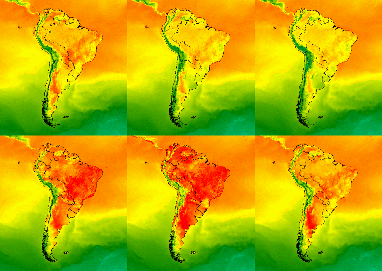
图 5. 向集合中的图片添加矢量叠加层,以提供空间背景信息。
图片叠层
您可以叠加多张图片,以达到理想的风格。假设您想强调某个感兴趣的区域。您可以创建图像可视化图表的静音副本作为基础层,然后叠加原始可视化图表的剪辑版本。基于上一个示例,以下脚本生成了图 6。
代码编辑器 (JavaScript)
// Define an empty image to paint features to.
var empty = ee.Image().byte();

// Paint country feature edges to the empty image.
var southAmOutline = empty
  .paint({featureCollection: southAmCol, color: 1, width: 1})
  // Convert to an RGB visualization image; set line color to black.
  .visualize({palette: '000000'});

// Map a blend operation over the temperature collection to overlay the country
// border outline image on all collection images.
var tempColOutline = tempColVis.map(function(img) {
  return img.blend(southAmOutline);
});

// Define a partially opaque grey RGB image to dull the underlying image when
// blended as an overlay.
var dullLayer = ee.Image.constant(175).visualize({
  opacity: 0.6, min: 0, max: 255, forceRgbOutput: true});

// Map a two-part blending operation over the country outline temperature
// collection for final styling.
var finalVisCol = tempColOutline.map(function(img) {
  return img
    // Blend the dulling layer with the given country outline temperature image.
    .blend(dullLayer)
    // Blend a clipped copy of the country outline temperature image with the
    // dulled background image.
    .blend(img.clipToCollection(southAmCol));
});

// Define animation arguments.
var videoArgs = {
  dimensions: 768,
  region: southAmAoi,
  framesPerSecond: 7,
  crs: 'EPSG:3857'
};

// Display the animation.
print(ui.Thumbnail(finalVisCol, videoArgs));
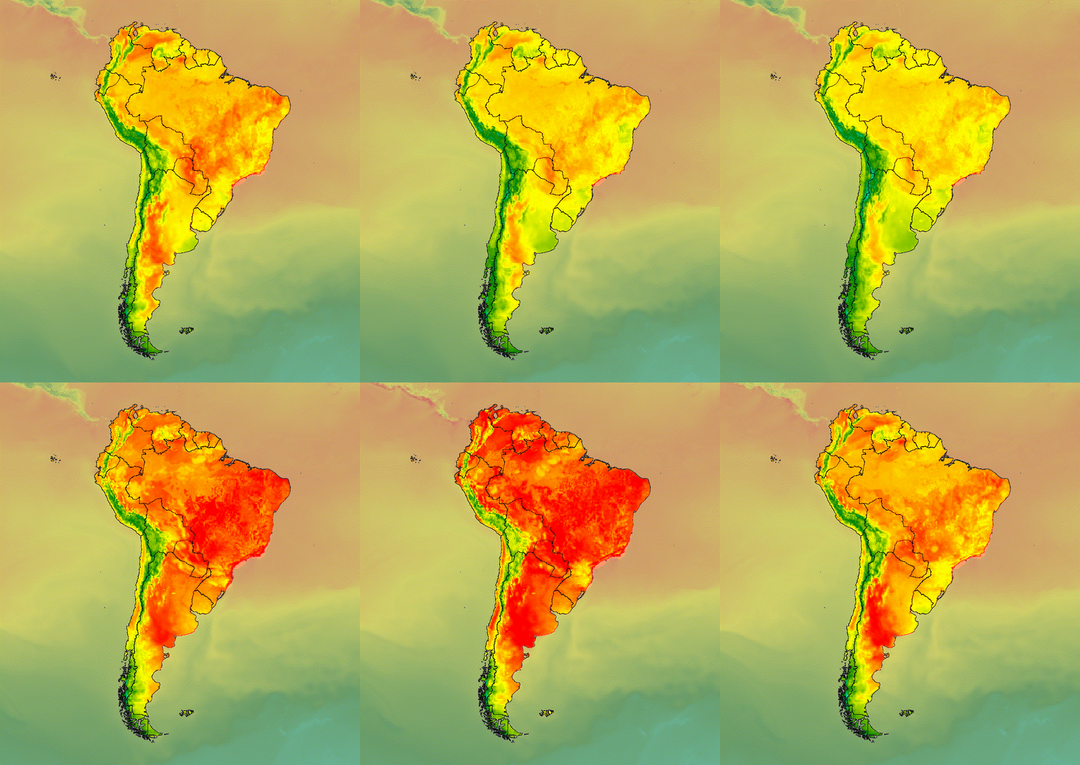
图 6. 通过剪辑图片并将其叠加在静音副本上,强调感兴趣的区域。
您还可以将图像数据与山体阴影基础图层混合,以指示地形并为可视化效果提供一定的深度(图 7)。
代码编辑器 (JavaScript)
// Define a hillshade layer from NASADEM digital elevation model.
var hillshade = ee.Terrain.hillshade(ee.Image('NASA/NASADEM_HGT/001')
  // Exaggerate the elevation to increase contrast in hillshade.
  .multiply(100))
  // Clip the DEM by South American boundary to clean boundary between
  // land and ocean.
  .clipToCollection(southAmCol);

// Map a blend operation over the temperature collection to overlay a partially
// opaque temperature layer on the hillshade layer.
var finalVisCol = tempColVis.map(function(img) {
  return hillshade
    .blend(img.clipToCollection(southAmCol).visualize({opacity: 0.6}));
});

// Define animation arguments.
var videoArgs = {
  dimensions: 768,
  region: southAmAoi,
  framesPerSecond: 7,
  crs: 'EPSG:3857'
};

// Display the animation.
print(ui.Thumbnail(finalVisCol, videoArgs));
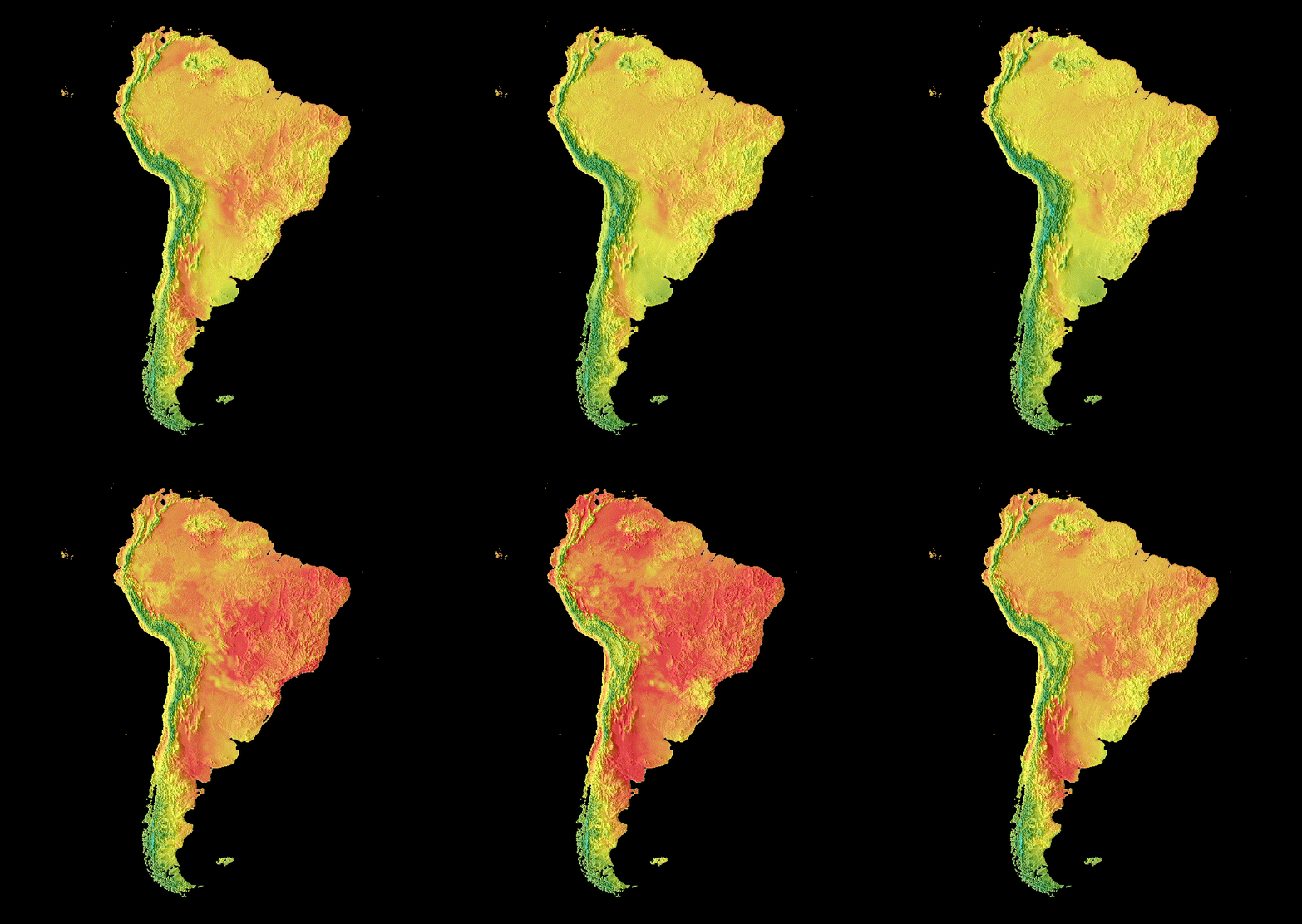
图 7. 通过在山体阴影图层上叠加半透明图片数据来显示地形。
转场效果
自定义图片集合,以生成动画,通过淡入淡出、闪烁和滑动过渡来显示集合中两张图片之间的差异。以下每个示例都使用由以下脚本生成的相同基本可视化图表:
代码编辑器 (JavaScript)
// Define an area of interest geometry with a global non-polar extent.
var aoi = ee.Geometry.Polygon(
  [[[-179.0, 78.0], [-179.0, -58.0], [179.0, -58.0], [179.0, 78.0]]], null,
  false);

// Import hourly predicted temperature image collection.
var temp = ee.ImageCollection('NOAA/GFS0P25')

// Define a northern summer solstice temperature image.
var summerSolTemp = temp
  .filterDate('2018-06-21', '2018-06-22')
  .filterMetadata('forecast_hours', 'equals', 12)
  .first()
  .select('temperature_2m_above_ground');

// Define a northern winter solstice temperature image.
var winterSolTemp = temp
  .filterDate('2018-12-22', '2018-12-23')
  .filterMetadata('forecast_hours', 'equals', 12)
  .first()
  .select('temperature_2m_above_ground');

// Combine the solstice images into a collection.
var tempCol = ee.ImageCollection([
  summerSolTemp.set('season', 'summer'),
  winterSolTemp.set('season', 'winter')
]);

// Import international boundaries feature collection.
var countries = ee.FeatureCollection('USDOS/LSIB_SIMPLE/2017');

// Define visualization arguments.
var visArgs = {
  min: -40.0,
  max: 35.0,
  palette: ['blue', 'purple', 'cyan', 'green', 'yellow', 'red']
};

// Convert the image data to RGB visualization images.
// The clip and unmask combination sets ocean pixels to black.
var tempColVis = tempCol.map(function(img) {
  return img
    .visualize(visArgs)
    .clipToCollection(countries)
    .unmask(0)
    .copyProperties(img, img.propertyNames());
});
闪烁
如果集合中只有两张图片(如此处所示),则闪烁是集合动画的默认表示形式。调整 framesPerSecond 动画参数,以加快或减慢闪烁速率。将以下可视化参数应用于上述集合,会生成图 8。
代码编辑器 (JavaScript)
// Define arguments for animation function parameters.
var videoArgs = {
  dimensions: 768,
  region: aoi,
  framesPerSecond: 2,
  crs: 'EPSG:3857'
};

// Display animation to the Code Editor console.
print(ui.Thumbnail(tempColVis, videoArgs));
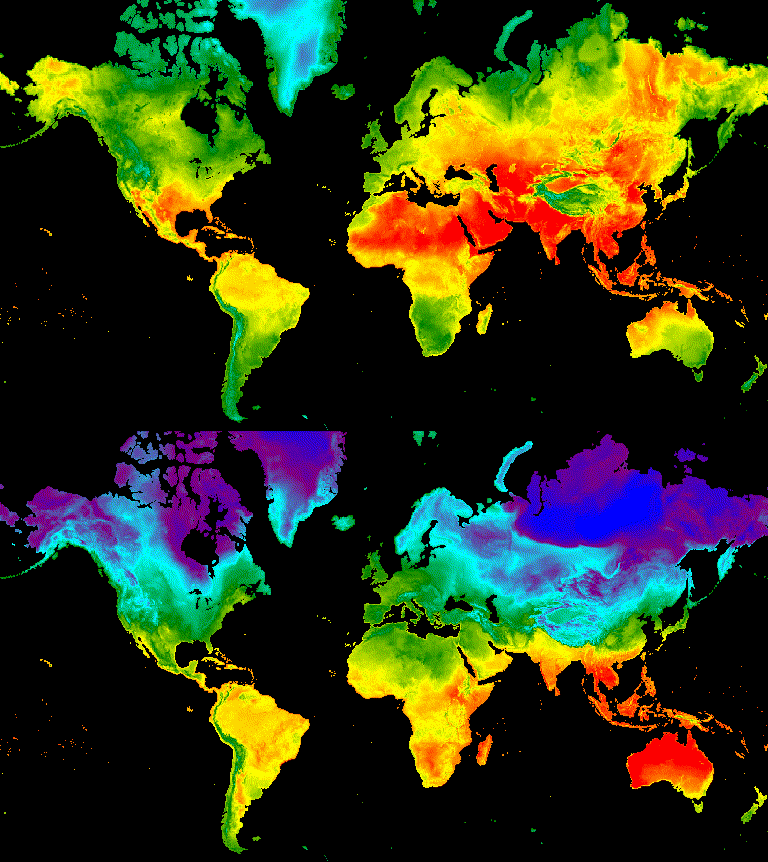
图 8. 示例:格林尼治标准时间中午 12 点的北半球夏至和冬至地表温度交替显示。
淡化
两个图层之间的淡入淡出过渡是通过在不透明度从接近 0 到 1 的一系列增量中,同时降低一个图层的不透明度并提高另一个图层的不透明度来实现的(图 9)。
代码编辑器 (JavaScript)
// Define a sequence of decreasing opacity increments. Note that opacity cannot
// be 0, so near 1 and 0 are used. Near 1 is needed because a compliment is
// calculated in a following step that can result in 0 if 1 is an element of the
// list.
var opacityList = ee.List.sequence({start: 0.99999, end: 0.00001, count: 20});

// Filter the summer and winter solstice images from the collection and set as
// image objects.
var summerImg = tempColVis.filter(ee.Filter.eq('season', 'summer')).first();
var winterImg = tempColVis.filter(ee.Filter.eq('season', 'winter')).first();

// Map over the list of opacity increments to iteratively adjust the opacity of
// the two solstice images. Returns a list of images.
var imgList = opacityList.map(function(opacity) {
  var opacityCompliment = ee.Number(1).subtract(ee.Number(opacity));
  var winterImgFade = winterImg.visualize({opacity: opacity});
  var summerImgFade = summerImg.visualize({opacity: opacityCompliment});
  return summerImgFade.blend(winterImgFade).set('opacity', opacity);
});

// Convert the image list to an image collection; the forward phase.
var fadeForward = ee.ImageCollection.fromImages(imgList);

// Make a copy of the collection that is sorted by ascending opacity to
// represent the reverse phase.
var fadeBackward = fadeForward.sort({property: 'opacity'});

// Merge the forward and reverse phase frame collections.
var fadeCol = fadeForward.merge(fadeBackward);

// Define animation arguments.
var videoArgs = {
  dimensions: 768,
  region: aoi,
  framesPerSecond: 25,
  crs: 'EPSG:3857'
};

// Display the animation.
print(ui.Thumbnail(fadeCol, videoArgs));
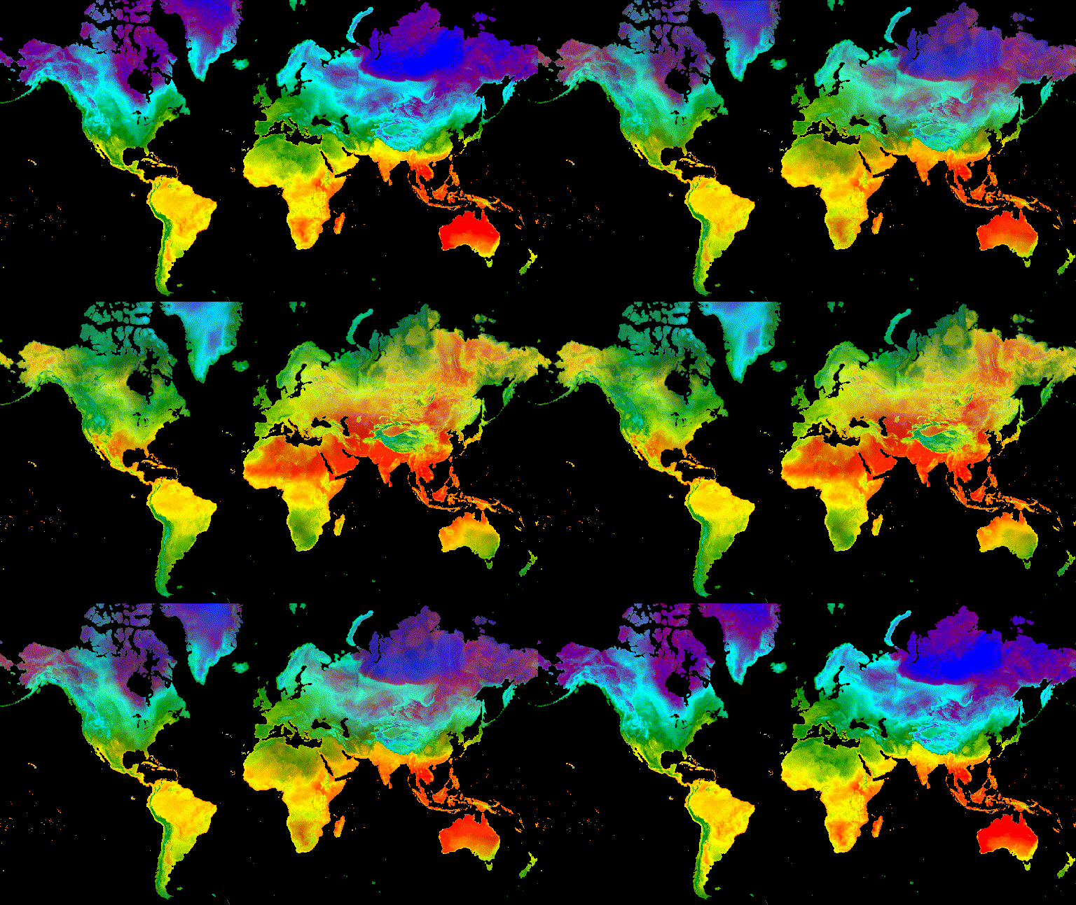
图 9. 示例:夏至和冬至格林尼治标准时间中午 12 点地表温度之间的渐变。
滑块
滑块过渡效果会逐渐显示和隐藏底层图片层。 这是通过在一定经度范围内迭代调整叠加图像的不透明度来实现的(图 10)。
代码编辑器 (JavaScript)
// Define a sequence of longitude increments. Start and end are defined by the
// min and max longitude of the feature to be provided to the region parameter
// of the animation arguments dictionary.
var lonSeq = ee.List.sequence({start: -179, end: 179, count: 20});

// Define a longitude image.
var longitude = ee.Image.pixelLonLat().select('longitude');

// Filter the summer and winter solstice images from the collection and set as
// image objects.
var summerImg = tempColVis.filter(ee.Filter.eq('season', 'summer')).first();
var winterImg = tempColVis.filter(ee.Filter.eq('season', 'winter')).first();

// Map over the list of longitude increments to iteratively adjust the mask
// (opacity) of the overlying image layer. Returns a list of images.
var imgList = lonSeq.map(function(lon) {
  lon = ee.Number(lon);
  var mask = longitude.gt(lon);
  return summerImg.blend(winterImg.updateMask(mask)).set('lon', lon);
});

// Convert the image list to an image collection; concealing phase.
var sliderColForward = ee.ImageCollection.fromImages(imgList);

// Make a copy of the collection that is sorted by descending longitude to
// represent the revealing phase.
var sliderColbackward = sliderColForward
  .sort({property: 'lon', ascending: false});

// Merge the forward and backward phase frame collections.
var sliderCol = sliderColForward.merge(sliderColbackward);

// Define animation arguments.
var videoArgs = {
  dimensions: 768,
  region: aoi,
  framesPerSecond: 25,
  crs: 'EPSG:3857'
};

// Display the animation.
print(ui.Thumbnail(sliderCol, videoArgs));
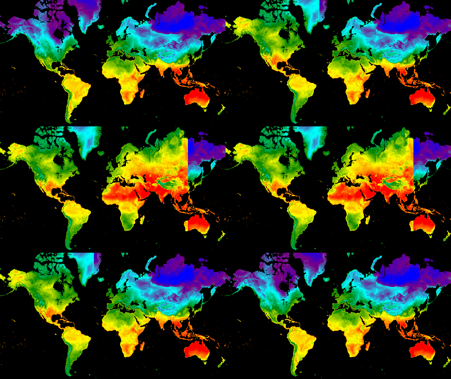
图 10. 夏至和冬至格林尼治标准时间中午 12 点地表温度之间的滑动过渡示例。