 在 GitHub 上查看源代码
有许多 ee.Image 方法可生成图片数据的 RGB 可视化表示,例如:visualize()、getThumbURL()、getMap()、getMapId()(用于 Colab Folium 地图显示)和 Map.addLayer()(用于代码编辑器地图显示,不适用于 Python)。默认情况下,这些方法会将前三个波段分别分配给红色、绿色和蓝色。默认的伸展取决于波段中数据的类型(例如,浮点数会在 [0, 1] 范围内进行伸展,16 位数据会被伸展到可能值的整个范围),这可能或许不适合。如需实现所需的可视化效果,您可以提供可视化参数:
| 参数 | 说明 | 类型 |
|---|---|---|
| 乐队 | 要映射到 RGB 的三个波段名称的逗号分隔列表 | list |
| 分钟 | 要映射到 0 的值 | 一个数字或三个数字的列表,每个频段对应一个数字 |
| 最大值 | 要映射到 255 的值 | 一个数字或三个数字的列表,每个频段对应一个数字 |
| gain | 用于将每个像素值乘以的值 | 一个数字或三个数字的列表,每个频段对应一个数字 |
| 偏差 | 要添加到每个 DN 的值 | 一个数字或三个数字的列表,每个频段对应一个数字 |
| gamma | 伽玛校正系数 | 一个数字或三个数字的列表,每个频段对应一个数字 |
| palette | CSS 样式颜色字符串列表(仅限单波段图片) | 以英文逗号分隔的十六进制字符串列表 |
| 不透明度 | 图层的不透明度(0.0 表示完全透明,1.0 表示完全不透明) | 数值 |
| format | “jpg”或“png” | 字符串 |
RGB 合成
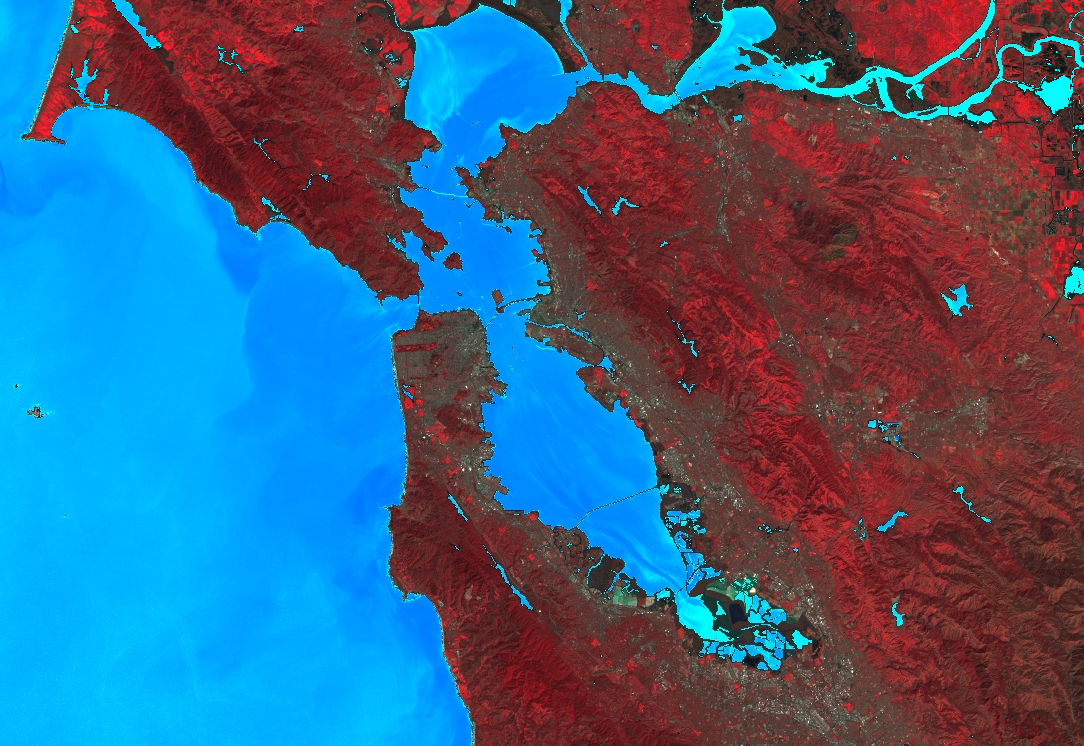
以下示例展示了如何使用参数将 Landsat 8 图片的样式设置为假彩色合成图:
Code Editor (JavaScript)
// Load an image.
var image = ee.Image('LANDSAT/LC08/C02/T1_TOA/LC08_044034_20140318');

// Define the visualization parameters.
var vizParams = {
  bands: ['B5', 'B4', 'B3'],
  min: 0,
  max: 0.5,
  gamma: [0.95, 1.1, 1]
};

// Center the map and display the image.
Map.setCenter(-122.1899, 37.5010, 10); // San Francisco Bay
Map.addLayer(image, vizParams, 'false color composite');
import ee
import geemap.core as geemap
Colab (Python)
# Load an image.
image = ee.Image('LANDSAT/LC08/C02/T1_TOA/LC08_044034_20140318')

# Define the visualization parameters.
image_viz_params = {
    'bands': ['B5', 'B4', 'B3'],
    'min': 0,
    'max': 0.5,
    'gamma': [0.95, 1.1, 1],
}

# Define a map centered on San Francisco Bay.
map_l8 = geemap.Map(center=[37.5010, -122.1899], zoom=10)

# Add the image layer to the map and display it.
map_l8.add_layer(image, image_viz_params, 'false color composite')
display(map_l8)
在此示例中,'B5' 频段分配为红色,'B4' 分配为绿色,'B3' 分配为蓝色。

调色板
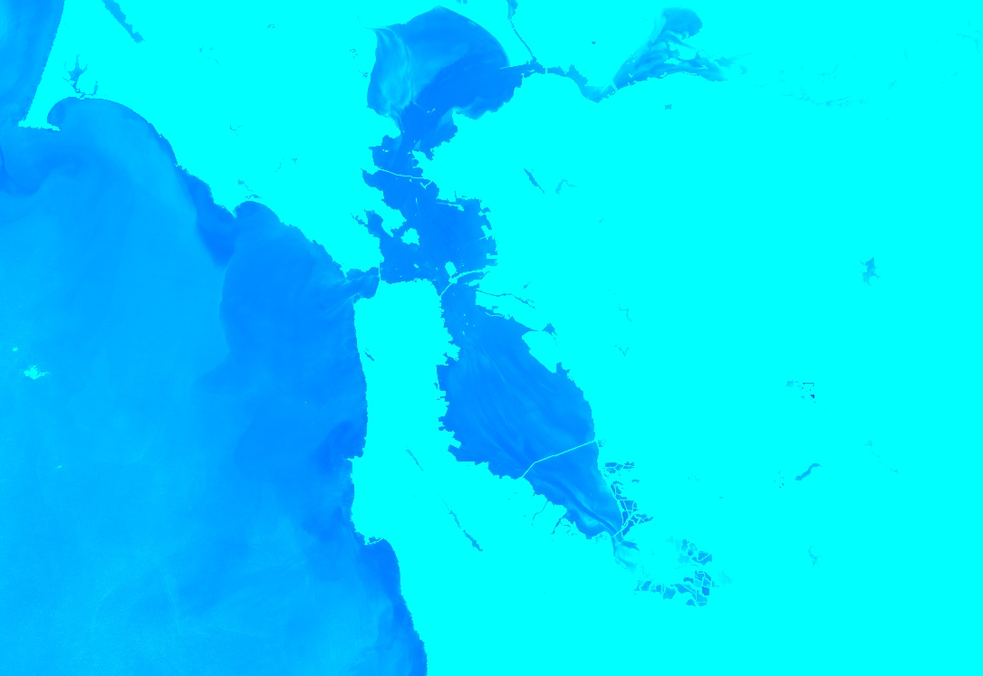
如需以颜色显示图片的单个波段,请使用由 CSS 样式的颜色字符串列表表示的颜色梯度设置 palette 参数。(如需了解详情,请参阅此参考文档)。以下示例展示了如何使用从青色 ('00FFFF') 到蓝色 ('0000FF') 的颜色来渲染
归一化差异水量指数 (NDWI) 图像:
Code Editor (JavaScript)
// Load an image.
var image = ee.Image('LANDSAT/LC08/C02/T1_TOA/LC08_044034_20140318');

// Create an NDWI image, define visualization parameters and display.
var ndwi = image.normalizedDifference(['B3', 'B5']);
var ndwiViz = {min: 0.5, max: 1, palette: ['00FFFF', '0000FF']};
Map.addLayer(ndwi, ndwiViz, 'NDWI', false);
import ee
import geemap.core as geemap
Colab (Python)
# Load an image.
image = ee.Image('LANDSAT/LC08/C02/T1_TOA/LC08_044034_20140318')

# Create an NDWI image, define visualization parameters and display.
ndwi = image.normalizedDifference(['B3', 'B5'])
ndwi_viz = {'min': 0.5, 'max': 1, 'palette': ['00FFFF', '0000FF']}

# Define a map centered on San Francisco Bay.
map_ndwi = geemap.Map(center=[37.5010, -122.1899], zoom=10)

# Add the image layer to the map and display it.
map_ndwi.add_layer(ndwi, ndwi_viz, 'NDWI')
display(map_ndwi)
在此示例中,请注意 min 和 max 参数表示应应用调色板的像素值范围。中间值会线性拉伸。
另请注意,在代码编辑器示例中,show 参数设置为 false。这会导致图层在添加到地图后处于不可见状态。您可以随时使用代码编辑器地图右上角的图层管理器重新开启该功能。
遮盖
您可以使用 image.updateMask() 根据遮罩图片中非零像素的位置设置单个像素的不透明度。系统会将遮罩中等于零的像素从计算中排除,并将不透明度设置为 0 以进行显示。以下示例使用 NDWI 阈值(如需了解阈值,请参阅
“关系运算”部分)更新之前创建的 NDWI 图层上的掩码:
Code Editor (JavaScript)
// Mask the non-watery parts of the image, where NDWI < 0.4.
var ndwiMasked = ndwi.updateMask(ndwi.gte(0.4));
Map.addLayer(ndwiMasked, ndwiViz, 'NDWI masked');
import ee
import geemap.core as geemap
Colab (Python)
# Mask the non-watery parts of the image, where NDWI < 0.4.
ndwi_masked = ndwi.updateMask(ndwi.gte(0.4))

# Define a map centered on San Francisco Bay.
map_ndwi_masked = geemap.Map(center=[37.5010, -122.1899], zoom=10)

# Add the image layer to the map and display it.
map_ndwi_masked.add_layer(ndwi_masked, ndwi_viz, 'NDWI masked')
display(map_ndwi_masked)
可视化图片
使用 image.visualize() 方法将图片转换为 8 位 RGB 图片,以便显示或导出。例如,如需将假彩合成图和 NDWI 转换为 3 波段显示图像,请使用以下命令:
Code Editor (JavaScript)
// Create visualization layers.
var imageRGB = image.visualize({bands: ['B5', 'B4', 'B3'], max: 0.5});
var ndwiRGB = ndwiMasked.visualize({
  min: 0.5,
  max: 1,
  palette: ['00FFFF', '0000FF']
});
import ee
import geemap.core as geemap
Colab (Python)
image_rgb = image.visualize(bands=['B5', 'B4', 'B3'], max=0.5)
ndwi_rgb = ndwi_masked.visualize(min=0.5, max=1, palette=['00FFFF', '0000FF'])
马赛克
您可以使用遮盖和 imageCollection.mosaic()(如需了解如何拼接,请参阅“拼接”部分)来实现各种地图效果。mosaic() 方法会根据图层在输入集合中的顺序渲染输出图片中的图层。以下示例使用 mosaic() 组合经过掩码的 NDWI 和假彩色合成图,并获得新的可视化结果:
Code Editor (JavaScript)
// Mosaic the visualization layers and display (or export).
var mosaic = ee.ImageCollection([imageRGB, ndwiRGB]).mosaic();
Map.addLayer(mosaic, {}, 'mosaic');
import ee
import geemap.core as geemap
Colab (Python)
# Mosaic the visualization layers and display (or export).
mosaic = ee.ImageCollection([image_rgb, ndwi_rgb]).mosaic()

# Define a map centered on San Francisco Bay.
map_mosaic = geemap.Map(center=[37.5010, -122.1899], zoom=10)

# Add the image layer to the map and display it.
map_mosaic.add_layer(mosaic, None, 'mosaic')
display(map_mosaic)
在此示例中,请注意,系统会向 ImageCollection 构造函数提供两个可视化图片的列表。列表的顺序决定了图片在地图上的呈现顺序。
剪裁
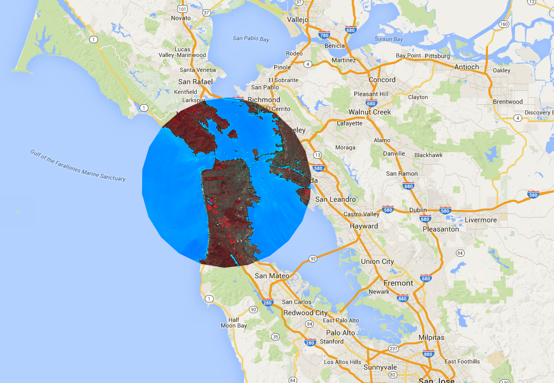
image.clip() 方法对于实现地图效果非常有用。以下示例将之前创建的拼接图剪裁到旧金山市周围的任意缓冲区:
Code Editor (JavaScript)
// Create a circle by drawing a 20000 meter buffer around a point.
var roi = ee.Geometry.Point([-122.4481, 37.7599]).buffer(20000);

// Display a clipped version of the mosaic.
Map.addLayer(mosaic.clip(roi), null, 'mosaic clipped');
import ee
import geemap.core as geemap
Colab (Python)
# Create a circle by drawing a 20000 meter buffer around a point.
roi = ee.Geometry.Point([-122.4481, 37.7599]).buffer(20000)
mosaic_clipped = mosaic.clip(roi)

# Define a map centered on San Francisco.
map_mosaic_clipped = geemap.Map(center=[37.7599, -122.4481], zoom=10)

# Add the image layer to the map and display it.
map_mosaic_clipped.add_layer(mosaic_clipped, None, 'mosaic clipped')
display(map_mosaic_clipped)
请注意,在上面的示例中,坐标会提供给 Geometry 构造函数,并且缓冲区长度指定为 2 万米。如需详细了解几何图形,请参阅“几何图形”页面。
渲染分类地图
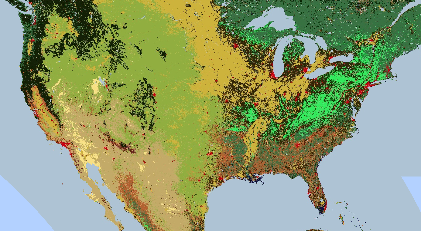
调色板还适用于渲染离散值地图,例如土地覆盖地图。
如果有多个类,请使用调色板为每个类提供不同的颜色。
(在这种情况下,image.remap() 方法可能很有用,可将任意标签转换为连续整数)。以下示例使用调色板渲染土地覆盖类别:
Code Editor (JavaScript)
// Load 2012 MODIS land cover and select the IGBP classification.
var cover = ee.Image('MODIS/051/MCD12Q1/2012_01_01')
  .select('Land_Cover_Type_1');

// Define a palette for the 18 distinct land cover classes.
var igbpPalette = [
  'aec3d4', // water
  '152106', '225129', '369b47', '30eb5b', '387242', // forest
  '6a2325', 'c3aa69', 'b76031', 'd9903d', '91af40',  // shrub, grass
  '111149', // wetlands
  'cdb33b', // croplands
  'cc0013', // urban
  '33280d', // crop mosaic
  'd7cdcc', // snow and ice
  'f7e084', // barren
  '6f6f6f'  // tundra
];

// Specify the min and max labels and the color palette matching the labels.
Map.setCenter(-99.229, 40.413, 5);
Map.addLayer(cover,
             {min: 0, max: 17, palette: igbpPalette},
             'IGBP classification');
import ee
import geemap.core as geemap
Colab (Python)
# Load 2012 MODIS land cover and select the IGBP classification.
cover = ee.Image('MODIS/051/MCD12Q1/2012_01_01').select('Land_Cover_Type_1')

# Define a palette for the 18 distinct land cover classes.
igbp_palette = [
    'aec3d4',  # water
    '152106',
    '225129',
    '369b47',
    '30eb5b',
    '387242',  # forest
    '6a2325',
    'c3aa69',
    'b76031',
    'd9903d',
    '91af40',  # shrub, grass
    '111149',  # wetlands
    'cdb33b',  # croplands
    'cc0013',  # urban
    '33280d',  # crop mosaic
    'd7cdcc',  # snow and ice
    'f7e084',  # barren
    '6f6f6f',  # tundra
]

# Define a map centered on the United States.
map_palette = geemap.Map(center=[40.413, -99.229], zoom=5)

# Add the image layer to the map and display it. Specify the min and max labels
# and the color palette matching the labels.
map_palette.add_layer(
    cover, {'min': 0, 'max': 17, 'palette': igbp_palette}, 'IGBP classes'
)
display(map_palette)
样式化图层描述符
您可以使用样式图层描述符 (SLD) 渲染要显示的图像。为 image.sldStyle() 提供图片符号化和着色的 XML 说明,具体而言是 RasterSymbolizer 元素。如需详细了解 RasterSymbolizer 元素,请点击此处。
例如,如需使用 SLD 渲染“渲染分类地图”部分中所述的土地覆盖地图,请使用以下代码:
Code Editor (JavaScript)
var cover = ee.Image('MODIS/051/MCD12Q1/2012_01_01').select('Land_Cover_Type_1');

// Define an SLD style of discrete intervals to apply to the image.
var sld_intervals =
'<RasterSymbolizer>' +
  '<ColorMap type="intervals" extended="false">' +
    '<ColorMapEntry color="#aec3d4" quantity="0" label="Water"/>' +
    '<ColorMapEntry color="#152106" quantity="1" label="Evergreen Needleleaf Forest"/>' +
    '<ColorMapEntry color="#225129" quantity="2" label="Evergreen Broadleaf Forest"/>' +
    '<ColorMapEntry color="#369b47" quantity="3" label="Deciduous Needleleaf Forest"/>' +
    '<ColorMapEntry color="#30eb5b" quantity="4" label="Deciduous Broadleaf Forest"/>' +
    '<ColorMapEntry color="#387242" quantity="5" label="Mixed Deciduous Forest"/>' +
    '<ColorMapEntry color="#6a2325" quantity="6" label="Closed Shrubland"/>' +
    '<ColorMapEntry color="#c3aa69" quantity="7" label="Open Shrubland"/>' +
    '<ColorMapEntry color="#b76031" quantity="8" label="Woody Savanna"/>' +
    '<ColorMapEntry color="#d9903d" quantity="9" label="Savanna"/>' +
    '<ColorMapEntry color="#91af40" quantity="10" label="Grassland"/>' +
    '<ColorMapEntry color="#111149" quantity="11" label="Permanent Wetland"/>' +
    '<ColorMapEntry color="#cdb33b" quantity="12" label="Cropland"/>' +
    '<ColorMapEntry color="#cc0013" quantity="13" label="Urban"/>' +
    '<ColorMapEntry color="#33280d" quantity="14" label="Crop, Natural Veg. Mosaic"/>' +
    '<ColorMapEntry color="#d7cdcc" quantity="15" label="Permanent Snow, Ice"/>' +
    '<ColorMapEntry color="#f7e084" quantity="16" label="Barren, Desert"/>' +
    '<ColorMapEntry color="#6f6f6f" quantity="17" label="Tundra"/>' +
  '</ColorMap>' +
'</RasterSymbolizer>';
Map.addLayer(cover.sldStyle(sld_intervals), {}, 'IGBP classification styled');
import ee
import geemap.core as geemap
Colab (Python)
cover = ee.Image('MODIS/051/MCD12Q1/2012_01_01').select('Land_Cover_Type_1')

# Define an SLD style of discrete intervals to apply to the image.
sld_intervals = """
<RasterSymbolizer>
  <ColorMap  type="intervals" extended="false" >
    <ColorMapEntry color="#aec3d4" quantity="0" label="Water"/>
    <ColorMapEntry color="#152106" quantity="1" label="Evergreen Needleleaf Forest"/>
    <ColorMapEntry color="#225129" quantity="2" label="Evergreen Broadleaf Forest"/>
    <ColorMapEntry color="#369b47" quantity="3" label="Deciduous Needleleaf Forest"/>
    <ColorMapEntry color="#30eb5b" quantity="4" label="Deciduous Broadleaf Forest"/>
    <ColorMapEntry color="#387242" quantity="5" label="Mixed Deciduous Forest"/>
    <ColorMapEntry color="#6a2325" quantity="6" label="Closed Shrubland"/>
    <ColorMapEntry color="#c3aa69" quantity="7" label="Open Shrubland"/>
    <ColorMapEntry color="#b76031" quantity="8" label="Woody Savanna"/>
    <ColorMapEntry color="#d9903d" quantity="9" label="Savanna"/>
    <ColorMapEntry color="#91af40" quantity="10" label="Grassland"/>
    <ColorMapEntry color="#111149" quantity="11" label="Permanent Wetland"/>
    <ColorMapEntry color="#cdb33b" quantity="12" label="Cropland"/>
    <ColorMapEntry color="#cc0013" quantity="13" label="Urban"/>
    <ColorMapEntry color="#33280d" quantity="14" label="Crop, Natural Veg. Mosaic"/>
    <ColorMapEntry color="#d7cdcc" quantity="15" label="Permanent Snow, Ice"/>
    <ColorMapEntry color="#f7e084" quantity="16" label="Barren, Desert"/>
    <ColorMapEntry color="#6f6f6f" quantity="17" label="Tundra"/>
  </ColorMap>
</RasterSymbolizer>"""

# Apply the SLD style to the image.
cover_sld = cover.sldStyle(sld_intervals)

# Define a map centered on the United States.
map_sld_categorical = geemap.Map(center=[40.413, -99.229], zoom=5)

# Add the image layer to the map and display it.
map_sld_categorical.add_layer(cover_sld, None, 'IGBP classes styled')
display(map_sld_categorical)
如需创建带有颜色梯度的可视化图片,请将 ColorMap 的类型设置为“ramp”。以下示例比较了用于渲染 DEM 的“interval”和“ramp”类型:
Code Editor (JavaScript)
// Load SRTM Digital Elevation Model data.
var image = ee.Image('CGIAR/SRTM90_V4');

// Define an SLD style of discrete intervals to apply to the image. Use the
// opacity keyword to set pixels less than 0 as completely transparent. Pixels
// with values greater than or equal to the final entry quantity are set to
// fully transparent by default.
var sld_intervals =
  '<RasterSymbolizer>' +
    '<ColorMap type="intervals" extended="false" >' +
      '<ColorMapEntry color="#0000ff" quantity="0" label="0 ﹤ x" opacity="0" />' +
      '<ColorMapEntry color="#00ff00" quantity="100" label="0 ≤ x ﹤ 100" />' +
      '<ColorMapEntry color="#007f30" quantity="200" label="100 ≤ x ﹤ 200" />' +
      '<ColorMapEntry color="#30b855" quantity="300" label="200 ≤ x ﹤ 300" />' +
      '<ColorMapEntry color="#ff0000" quantity="400" label="300 ≤ x ﹤ 400" />' +
      '<ColorMapEntry color="#ffff00" quantity="900" label="400 ≤ x ﹤ 900" />' +
    '</ColorMap>' +
  '</RasterSymbolizer>';

// Define an sld style color ramp to apply to the image.
var sld_ramp =
  '<RasterSymbolizer>' +
    '<ColorMap type="ramp" extended="false" >' +
      '<ColorMapEntry color="#0000ff" quantity="0" label="0"/>' +
      '<ColorMapEntry color="#00ff00" quantity="100" label="100" />' +
      '<ColorMapEntry color="#007f30" quantity="200" label="200" />' +
      '<ColorMapEntry color="#30b855" quantity="300" label="300" />' +
      '<ColorMapEntry color="#ff0000" quantity="400" label="400" />' +
      '<ColorMapEntry color="#ffff00" quantity="500" label="500" />' +
    '</ColorMap>' +
  '</RasterSymbolizer>';

// Add the image to the map using both the color ramp and interval schemes.
Map.setCenter(-76.8054, 42.0289, 8);
Map.addLayer(image.sldStyle(sld_intervals), {}, 'SLD intervals');
Map.addLayer(image.sldStyle(sld_ramp), {}, 'SLD ramp');
import ee
import geemap.core as geemap
Colab (Python)
# Load SRTM Digital Elevation Model data.
image = ee.Image('CGIAR/SRTM90_V4')

# Define an SLD style of discrete intervals to apply to the image.
sld_intervals = """
    <RasterSymbolizer>
      <ColorMap type="intervals" extended="false" >
        <ColorMapEntry color="#0000ff" quantity="0" label="0"/>
        <ColorMapEntry color="#00ff00" quantity="100" label="1-100" />
        <ColorMapEntry color="#007f30" quantity="200" label="110-200" />
        <ColorMapEntry color="#30b855" quantity="300" label="210-300" />
        <ColorMapEntry color="#ff0000" quantity="400" label="310-400" />
        <ColorMapEntry color="#ffff00" quantity="1000" label="410-1000" />
      </ColorMap>
    </RasterSymbolizer>"""

# Define an sld style color ramp to apply to the image.
sld_ramp = """
    <RasterSymbolizer>
      <ColorMap type="ramp" extended="false" >
        <ColorMapEntry color="#0000ff" quantity="0" label="0"/>
        <ColorMapEntry color="#00ff00" quantity="100" label="100" />
        <ColorMapEntry color="#007f30" quantity="200" label="200" />
        <ColorMapEntry color="#30b855" quantity="300" label="300" />
        <ColorMapEntry color="#ff0000" quantity="400" label="400" />
        <ColorMapEntry color="#ffff00" quantity="500" label="500" />
      </ColorMap>
    </RasterSymbolizer>"""

# Define a map centered on the United States.
map_sld_interval = geemap.Map(center=[40.413, -99.229], zoom=5)

# Add the image layers to the map and display it.
map_sld_interval.add_layer(
    image.sldStyle(sld_intervals), None, 'SLD intervals'
)
map_sld_interval.add_layer(image.sldStyle(sld_ramp), None, 'SLD ramp')
display(map_sld_interval)
SLD 还可用于拉伸像素值,以改进连续数据的可视化效果。例如,以下代码比较了任意线性拉伸与最小-最大“标准化”和“直方图”均衡的结果:
Code Editor (JavaScript)
// Load a Landsat 8 raw image.
var image = ee.Image('LANDSAT/LC08/C02/T1/LC08_044034_20140318');

// Define a RasterSymbolizer element with '_enhance_' for a placeholder.
var template_sld =
  '<RasterSymbolizer>' +
    '<ContrastEnhancement><_enhance_/></ContrastEnhancement>' +
    '<ChannelSelection>' +
      '<RedChannel>' +
        '<SourceChannelName>B5</SourceChannelName>' +
      '</RedChannel>' +
      '<GreenChannel>' +
        '<SourceChannelName>B4</SourceChannelName>' +
      '</GreenChannel>' +
      '<BlueChannel>' +
        '<SourceChannelName>B3</SourceChannelName>' +
      '</BlueChannel>' +
    '</ChannelSelection>' +
  '</RasterSymbolizer>';

// Get SLDs with different enhancements.
var equalize_sld = template_sld.replace('_enhance_', 'Histogram');
var normalize_sld = template_sld.replace('_enhance_', 'Normalize');

// Display the results.
Map.centerObject(image, 10);
Map.addLayer(image, {bands: ['B5', 'B4', 'B3'], min: 0, max: 15000}, 'Linear');
Map.addLayer(image.sldStyle(equalize_sld), {}, 'Equalized');
Map.addLayer(image.sldStyle(normalize_sld), {}, 'Normalized');
import ee
import geemap.core as geemap
Colab (Python)
# Load a Landsat 8 raw image.
image = ee.Image('LANDSAT/LC08/C02/T1/LC08_044034_20140318')

# Define a RasterSymbolizer element with '_enhance_' for a placeholder.
template_sld = """
<RasterSymbolizer>
  <ContrastEnhancement><_enhance_/></ContrastEnhancement>
  <ChannelSelection>
    <RedChannel>
      <SourceChannelName>B5</SourceChannelName>
    </RedChannel>
    <GreenChannel>
      <SourceChannelName>B4</SourceChannelName>
    </GreenChannel>
    <BlueChannel>
      <SourceChannelName>B3</SourceChannelName>
    </BlueChannel>
  </ChannelSelection>
</RasterSymbolizer>"""

# Get SLDs with different enhancements.
equalize_sld = template_sld.replace('_enhance_', 'Histogram')
normalize_sld = template_sld.replace('_enhance_', 'Normalize')

# Define a map centered on San Francisco Bay.
map_sld_continuous = geemap.Map(center=[37.5010, -122.1899], zoom=10)

# Add the image layers to the map and display it.
map_sld_continuous.add_layer(
    image, {'bands': ['B5', 'B4', 'B3'], 'min': 0, 'max': 15000}, 'Linear'
)
map_sld_continuous.add_layer(image.sldStyle(equalize_sld), None, 'Equalized')
map_sld_continuous.add_layer(
    image.sldStyle(normalize_sld), None, 'Normalized'
)
display(map_sld_continuous)
关于在 Earth Engine 中使用 SLD 的注意事项:
- 支持 OGC SLD 1.0 和 OGC SE 1.1。
- 传入的 XML 文档可以是完整的,也可以仅包含 RasterSymbolizer 元素及下方的元素。
- 您可以按 Earth Engine 名称或编号(“1”“2”等)选择波段。
- 浮点图像不支持直方图和归一化对比度拉伸机制。
- 只有当不透明度为 0.0(透明)时,系统才会将其纳入考量范围。非零不透明度值会被视为完全不透明。
- 系统目前会忽略 OverlapBehavior 定义。
- 目前不支持 ShadedRelief 机制。
- 目前不支持 ImageOutline 机制。
- 系统会忽略 Geometry 元素。
- 如果请求了直方图均衡或正则化,输出图片将包含 histogram_bandname 元数据。
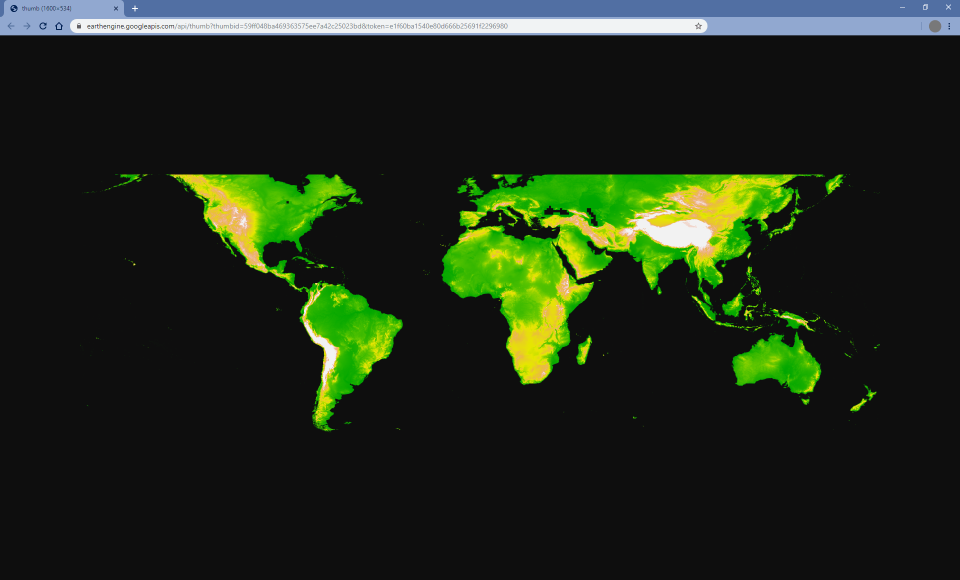
缩略图
使用 ee.Image.getThumbURL() 方法为 ee.Image 对象生成 PNG 或 JPEG 缩略图。输出以调用 getThumbURL() 结尾的表达式的结果会导致输出网址。访问该网址会将 Earth Engine 服务器设置为动态生成请求的缩略图。处理完成后,图片会显示在浏览器中。您可以通过从图片的右键点击上下文菜单中选择适当的选项来下载该图片。
getThumbURL() 方法包含上文可视化参数表中所述的参数。
此外,它还接受可选的 dimensions、region 和 crs 参数,用于控制缩略图的空间范围、大小和显示投影。
| 参数 | 说明 | 类型 |
|---|---|---|
| dimensions | 缩略图尺寸(以像素为单位)。如果只提供一个整数,则该整数会定义图片的较大宽高比维度的尺寸,并按比例缩放较小的维度。 默认为较大的图片宽高比,为 512 像素。 | 一个整数或字符串,格式为: 'WIDTHxHEIGHT' |
| 区域 | 要渲染的图片的地理区域。默认情况下是整个图片,或者是提供的几何图形的边界。 | GeoJSON 或至少包含三个点坐标的二维列表,用于定义线性环 |
| crs | 目标投影,例如“EPSG:3857”。默认为 WGS84(“EPSG:4326”)。 | 字符串 |
| format | 将缩略图格式定义为 PNG 或 JPEG。默认的 PNG 格式实现为 RGBA,其中 Alpha 通道表示有效和无效像素,由图片的 mask() 定义。无效像素是透明的。可选的 JPEG 格式以 RGB 格式实现,其中无效的图片像素会在 RGB 通道中填充零。
|
字符串;“png”或“jpg” |
单波段图像将默认设为灰度,除非您提供了 palette 参数。多波段图像将默认显示前三个波段的 RGB 可视化效果,除非您提供了 bands 参数。如果仅提供两个频段,第一个频段将映射到红色,第二个频段将映射到蓝色,而绿色通道将填充零。
以下是一系列示例,演示了 getThumbURL() 参数实参的各种组合。点击运行此脚本时输出的网址,即可查看缩略图。
Code Editor (JavaScript)
// Fetch a digital elevation model.
var image = ee.Image('CGIAR/SRTM90_V4');

// Request a default thumbnail of the DEM with defined linear stretch.
// Set masked pixels (ocean) to 1000 so they map as gray.
var thumbnail1 = image.unmask(1000).getThumbURL({
  'min': 0,
  'max': 3000,
  'dimensions': 500,
});
print('Default extent:', thumbnail1);

// Specify region by rectangle, define palette, set larger aspect dimension size.
var thumbnail2 = image.getThumbURL({
  'min': 0,
  'max': 3000,
  'palette': ['00A600','63C600','E6E600','E9BD3A','ECB176','EFC2B3','F2F2F2'],
  'dimensions': 500,
  'region': ee.Geometry.Rectangle([-84.6, -55.9, -32.9, 15.7]),
});
print('Rectangle region and palette:', thumbnail2);

// Specify region by a linear ring and set display CRS as Web Mercator.
var thumbnail3 = image.getThumbURL({
  'min': 0,
  'max': 3000,
  'palette': ['00A600','63C600','E6E600','E9BD3A','ECB176','EFC2B3','F2F2F2'],
  'region': ee.Geometry.LinearRing([[-84.6, 15.7], [-84.6, -55.9], [-32.9, -55.9]]),
  'dimensions': 500,
  'crs': 'EPSG:3857'
});
print('Linear ring region and specified crs', thumbnail3);
import ee
import geemap.core as geemap
Colab (Python)
# Fetch a digital elevation model.
image = ee.Image('CGIAR/SRTM90_V4')

# Request a default thumbnail of the DEM with defined linear stretch.
# Set masked pixels (ocean) to 1000 so they map as gray.
thumbnail_1 = image.unmask(1000).getThumbURL({
    'min': 0,
    'max': 3000,
    'dimensions': 500,
})
print('Default extent:', thumbnail_1)

# Specify region by rectangle, define palette, set larger aspect dimension size.
thumbnail_2 = image.getThumbURL({
    'min': 0,
    'max': 3000,
    'palette': [
        '00A600',
        '63C600',
        'E6E600',
        'E9BD3A',
        'ECB176',
        'EFC2B3',
        'F2F2F2',
    ],
    'dimensions': 500,
    'region': ee.Geometry.Rectangle([-84.6, -55.9, -32.9, 15.7]),
})
print('Rectangle region and palette:', thumbnail_2)

# Specify region by a linear ring and set display CRS as Web Mercator.
thumbnail_3 = image.getThumbURL({
    'min': 0,
    'max': 3000,
    'palette': [
        '00A600',
        '63C600',
        'E6E600',
        'E9BD3A',
        'ECB176',
        'EFC2B3',
        'F2F2F2',
    ],
    'region': ee.Geometry.LinearRing(
        [[-84.6, 15.7], [-84.6, -55.9], [-32.9, -55.9]]
    ),
    'dimensions': 500,
    'crs': 'EPSG:3857',
})
print('Linear ring region and specified crs:', thumbnail_3)