تتضمّن Earth Engine عدة طرق لإجراء الانحدار الخطي باستخدام عوامل الاختزال:
ee.Reducer.linearFit()ee.Reducer.linearRegression()ee.Reducer.robustLinearRegression()ee.Reducer.ridgeRegression()
أبسط طريقة لتقليل الانحدار الخطي هي linearFit() التي
تحسب تقدير التربيعات الأقل لدالة خطية لمتغيّر واحد مع
متغيّر ثابت. للحصول على نهج أكثر مرونة في وضع النماذج الخطية، استخدِم أحد
مُخفِّضات الانحدار الخطي التي تسمح بعدد متغيّر من
المتغيّرات المستقلة والتابعة. linearRegression() تنفِّذ نموذج الانحدار الخطي للمربّعات الصغرى العادية(OLS). تستخدِم robustLinearRegression() دالة تكلفة تستند
إلى المتبقيات من الانحدار لإزالة الوزن بشكل متكرّر من القيم الشاذة في البيانات
(O’Leary، 1990).
ينفِّذ ridgeRegression() الانحدار الخطي باستخدام أسلوب التطبيع L2.
إنّ تحليل الانحدار باستخدام هذه الطرق مناسب لتقليل
عناصر ee.ImageCollection وee.Image وee.FeatureCollection وee.List.
توضِّح الأمثلة التالية تطبيقًا لكل منها. يُرجى العلم أنّ
linearRegression() وrobustLinearRegression() وridgeRegression()
جميعها
تتضمّن بنية الإدخال والإخراج نفسها، ولكن يتوقعlinearFit() إدخالًا بنطاقين (X متبوعًا بـ Y) ويحتويridgeRegression() على مَعلمة إضافية (lambda، اختيارية) وإخراج (pValue).
ee.ImageCollection
linearFit()
يجب إعداد البيانات كصورة إدخال ذات نطاقين، حيث يكون النطاق الأول هو
المتغيّر المستقل والنطاق الثاني هو المتغيّر التابع. يوضّح المثال التالي تقدير المؤشر الخطي لهطول الأمطار في المستقبل (بعد عام 2006 في بيانات NEX-DCP30) الذي توقّعته نماذج المناخ. المتغيّر التابع هو هطول الأمطار المُتوقّع والمتغيّر المستقل هو الوقت، الذي تمت إضافته قبل استدعاء دالة
linearFit():
محرِّر الرموز البرمجية (JavaScript)
// This function adds a time band to the image.
var createTimeBand = function(image) {
  // Scale milliseconds by a large constant to avoid very small slopes
  // in the linear regression output.
  return image.addBands(image.metadata('system:time_start').divide(1e18));
};

// Load the input image collection: projected climate data.
var collection = ee.ImageCollection('NASA/NEX-DCP30_ENSEMBLE_STATS')
  .filter(ee.Filter.eq('scenario', 'rcp85'))
  .filterDate(ee.Date('2006-01-01'), ee.Date('2050-01-01'))
  // Map the time band function over the collection.
  .map(createTimeBand);

// Reduce the collection with the linear fit reducer.
// Independent variable are followed by dependent variables.
var linearFit = collection.select(['system:time_start', 'pr_mean'])
  .reduce(ee.Reducer.linearFit());

// Display the results.
Map.setCenter(-100.11, 40.38, 5);
Map.addLayer(linearFit,
  {min: 0, max: [-0.9, 8e-5, 1], bands: ['scale', 'offset', 'scale']}, 'fit');
يُرجى ملاحظة أنّ الإخراج يحتوي على شريطَين، وهما "الموضع المُعدَّل" (نقطة التقاطع) و"التدرّج" (يشير "التدرّج" في هذا السياق إلى ميل الخط، ولا ينبغي الخلط بينه وبين مَعلمة التدرّج التي يتم إدخالها في العديد من أدوات التقليل، والتي هي التدرّج المكاني). يجب أن تبدو النتيجة، التي تتضمّن مناطق ذات اتجاه متزايد باللون الأزرق، ومناطق ذات اتجاه متضائل باللون الأحمر ومناطق بدون اتجاه باللون الأخضر، على النحو الموضّح في الشكل 1.
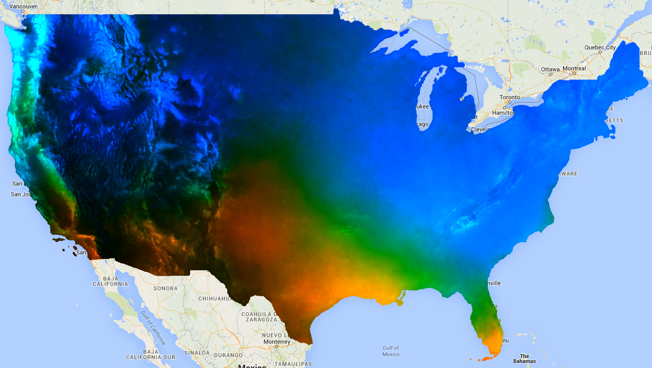
الشكل 1. الناتج من linearFit()
يتم تطبيقه على هطول الأمطار المتوقّع. تظهر المناطق التي يُتوقّع أن يزداد فيها معدل هطول الأمطار باللون الأزرق، والمناطق التي يُتوقّع أن ينخفض فيها معدل هطول الأمطار باللون الأحمر.
linearRegression()
على سبيل المثال، لنفترض أنّ هناك متغيرَين تابعَين: هطول الأمطار و أعلى درجة حرارة، ومتغيرَين مستقلَين: ثابت والوقت. المجموعة متطابقة مع المثال السابق، ولكن يجب إضافة النطاق الثابت يدويًا قبل التخفيض. الشريطَان الأولان من الإدخال هما المتغيّران "س" (مستقلان)، والشريبان التاليان هما المتغيّران "ص" (تابعان). في هذا المثال، احصل أولاً على صتيغ التراجُع، ثمّ اسطِح صورة المصفوفة لاستخراج النطاقات التي تهمّك:
محرِّر الرموز البرمجية (JavaScript)
// This function adds a time band to the image.
var createTimeBand = function(image) {
  // Scale milliseconds by a large constant.
  return image.addBands(image.metadata('system:time_start').divide(1e18));
};

// This function adds a constant band to the image.
var createConstantBand = function(image) {
  return ee.Image(1).addBands(image);
};

// Load the input image collection: projected climate data.
var collection = ee.ImageCollection('NASA/NEX-DCP30_ENSEMBLE_STATS')
  .filterDate(ee.Date('2006-01-01'), ee.Date('2099-01-01'))
  .filter(ee.Filter.eq('scenario', 'rcp85'))
  // Map the functions over the collection, to get constant and time bands.
  .map(createTimeBand)
  .map(createConstantBand)
  // Select the predictors and the responses.
  .select(['constant', 'system:time_start', 'pr_mean', 'tasmax_mean']);

// Compute ordinary least squares regression coefficients.
var linearRegression = collection.reduce(
  ee.Reducer.linearRegression({
    numX: 2,
    numY: 2
}));

// Compute robust linear regression coefficients.
var robustLinearRegression = collection.reduce(
  ee.Reducer.robustLinearRegression({
    numX: 2,
    numY: 2
}));

// The results are array images that must be flattened for display.
// These lists label the information along each axis of the arrays.
var bandNames = [['constant', 'time'], // 0-axis variation.
                 ['precip', 'temp']]; // 1-axis variation.

// Flatten the array images to get multi-band images according to the labels.
var lrImage = linearRegression.select(['coefficients']).arrayFlatten(bandNames);
var rlrImage = robustLinearRegression.select(['coefficients']).arrayFlatten(bandNames);

// Display the OLS results.
Map.setCenter(-100.11, 40.38, 5);
Map.addLayer(lrImage,
  {min: 0, max: [-0.9, 8e-5, 1], bands: ['time_precip', 'constant_precip', 'time_precip']}, 'OLS');

// Compare the results at a specific point:
print('OLS estimates:', lrImage.reduceRegion({
  reducer: ee.Reducer.first(),
  geometry: ee.Geometry.Point([-96.0, 41.0]),
  scale: 1000
}));

print('Robust estimates:', rlrImage.reduceRegion({
  reducer: ee.Reducer.first(),
  geometry: ee.Geometry.Point([-96.0, 41.0]),
  scale: 1000
}));
راجِع النتائج لمعرفة أنّ ناتج linearRegression() هو
معادل للمعاملات المقدَّرة من خلال المُخفِّض linearFit()، مع أنّه
يحتوي ناتج linearRegression() أيضًا على معاملات للمتغيّر المُستلَم الآخر، وهو tasmax_mean. تختلف معاملات الانحدار الخطي الفعّال عن
تقديرات OLS. يقارن المثال بين المعاملات من
طرق الانحدار المختلفة في نقطة معيّنة.
ee.Image
في سياق عنصر ee.Image، يمكن استخدام أدوات تقليل الانحدار مع
reduceRegion أو reduceRegions لإجراء انحدار خطي على وحدات البكسل في المناطق. توضِّح الأمثلة التالية
كيفية احتساب معاملات الانحدار بين نطاقات Landsat
في مضلّع عشوائي.
linearFit()
يعرض قسم الدليل الذي يصف مخططات بيانات المصفوفات
مخطّط انتشار للارتباط بين نطاقي SWIR1 وSWIR2
في Landsat 8. في ما يلي، يتم حساب معاملات الانحدار الخطي لهذه العلاقة. يتم عرض قاموس يحتوي على السمتَين 'offset' (نقطة تقاطع y) و
'scale' (المسافة المائلة).
محرِّر الرموز البرمجية (JavaScript)
// Define a rectangle geometry around San Francisco.
var sanFrancisco = ee.Geometry.Rectangle([-122.45, 37.74, -122.4, 37.8]);

// Import a Landsat 8 TOA image for this region.
var img = ee.Image('LANDSAT/LC08/C02/T1_TOA/LC08_044034_20140318');

// Subset the SWIR1 and SWIR2 bands. In the regression reducer, independent
// variables come first followed by the dependent variables. In this case,
// B5 (SWIR1) is the independent variable and B6 (SWIR2) is the dependent
// variable.
var imgRegress = img.select(['B5', 'B6']);

// Calculate regression coefficients for the set of pixels intersecting the
// above defined region using reduceRegion with ee.Reducer.linearFit().
var linearFit = imgRegress.reduceRegion({
  reducer: ee.Reducer.linearFit(),
  geometry: sanFrancisco,
  scale: 30,
});

// Inspect the results.
print('OLS estimates:', linearFit);
print('y-intercept:', linearFit.get('offset'));
print('Slope:', linearFit.get('scale'));
linearRegression()
يتم تطبيق التحليل نفسه من القسم السابق linearFit هنا،
باستثناء استخدام الدالة ee.Reducer.linearRegression هذه المرة. يُرجى العلم
أنّه يتم إنشاء صورة انحدار من ثلاث صور منفصلة: صورة
ثابتة وصور تمثّل نطاقي SWIR1 وSWIR2 من
صورة Landsat 8 نفسها. يُرجى العِلم أنّه يمكنك دمج أي مجموعة من النطاقات لإنشاء ملف تعريف
صورة لإدخالها في عملية تقليل المنطقة بنسبة ee.Reducer.linearRegression، ولا يجب أن تنتمي
هذه النطاقات إلى الصورة المصدر نفسها.
محرِّر الرموز البرمجية (JavaScript)
// Define a rectangle geometry around San Francisco.
var sanFrancisco = ee.Geometry.Rectangle([-122.45, 37.74, -122.4, 37.8]);

// Import a Landsat 8 TOA image for this region.
var img = ee.Image('LANDSAT/LC08/C02/T1_TOA/LC08_044034_20140318');

// Create a new image that is the concatenation of three images: a constant,
// the SWIR1 band, and the SWIR2 band.
var constant = ee.Image(1);
var xVar = img.select('B5');
var yVar = img.select('B6');
var imgRegress = ee.Image.cat(constant, xVar, yVar);

// Calculate regression coefficients for the set of pixels intersecting the
// above defined region using reduceRegion. The numX parameter is set as 2
// because the constant and the SWIR1 bands are independent variables and they
// are the first two bands in the stack; numY is set as 1 because there is only
// one dependent variable (SWIR2) and it follows as band three in the stack.
var linearRegression = imgRegress.reduceRegion({
  reducer: ee.Reducer.linearRegression({
    numX: 2,
    numY: 1
  }),
  geometry: sanFrancisco,
  scale: 30,
});

// Convert the coefficients array to a list.
var coefList = ee.Array(linearRegression.get('coefficients')).toList();

// Extract the y-intercept and slope.
var b0 = ee.List(coefList.get(0)).get(0); // y-intercept
var b1 = ee.List(coefList.get(1)).get(0); // slope

// Extract the residuals.
var residuals = ee.Array(linearRegression.get('residuals')).toList().get(0);

// Inspect the results.
print('OLS estimates', linearRegression);
print('y-intercept:', b0);
print('Slope:', b1);
print('Residuals:', residuals);
يتم عرض قاموس يحتوي على السمتَين 'coefficients' و'residuals'. السمة 'coefficients' هي مصفوفة بسمات
(numX, numY)، ويحتوي كل عمود على معاملات المتغيّر المرتبط
المقابل. في هذه الحالة، يحتوي الصفيف على صفين وعمود واحد، ويمثّل
الصف الأول، العمود الأول، قيمة "التقاطع مع محور السينات"، ويمثّل الصف الثاني، العمود الأول، قيمة "المسافة المائلة". سمة
'residuals' هي متجه جذر متوسط مربع المتبقيات لكل متغيّر تابع. استخرِج المعاملات من خلال تحويل النتيجة إلى صفيف، ثم استخرِج العناصر المطلوبة أو حوِّل الصفيف إلى قائمة واختَر المعاملات حسب موضع المؤشر.
ee.FeatureCollection
لنفترض أنّك تريد معرفة العلاقة الخطية بين انعكاس SWIR1 في Sentinel-2 و Landsat 8. في هذا المثال، يتم استخدام عيّنة عشوائية من البكسلات المُعدَّة كمجموعة ميزات من النقاط لاحتساب العلاقة. يتم إنشاء مخطّط مبعثر لزوجات وحدات البكسل مع خط أفضل تناسب باستخدام أقلّ مربعات (الشكل 2).
محرِّر الرموز البرمجية (JavaScript)
// Import a Sentinel-2 TOA image.
var s2ImgSwir1 = ee.Image('COPERNICUS/S2/20191022T185429_20191022T185427_T10SEH');

// Import a Landsat 8 TOA image from 12 days earlier than the S2 image.
var l8ImgSwir1 = ee.Image('LANDSAT/LC08/C02/T1_TOA/LC08_044033_20191010');

// Get the intersection between the two images - the area of interest (aoi).
var aoi = s2ImgSwir1.geometry().intersection(l8ImgSwir1.geometry());

// Get a set of 1000 random points from within the aoi. A feature collection
// is returned.
var sample = ee.FeatureCollection.randomPoints({
  region: aoi,
  points: 1000
});

// Combine the SWIR1 bands from each image into a single image.
var swir1Bands = s2ImgSwir1.select('B11')
  .addBands(l8ImgSwir1.select('B6'))
  .rename(['s2_swir1', 'l8_swir1']);

// Sample the SWIR1 bands using the sample point feature collection.
var imgSamp = swir1Bands.sampleRegions({
  collection: sample,
  scale: 30
})
// Add a constant property to each feature to be used as an independent variable.
.map(function(feature) {
  return feature.set('constant', 1);
});

// Compute linear regression coefficients. numX is 2 because
// there are two independent variables: 'constant' and 's2_swir1'. numY is 1
// because there is a single dependent variable: 'l8_swir1'. Cast the resulting
// object to an ee.Dictionary for easy access to the properties.
var linearRegression = ee.Dictionary(imgSamp.reduceColumns({
  reducer: ee.Reducer.linearRegression({
    numX: 2,
    numY: 1
  }),
  selectors: ['constant', 's2_swir1', 'l8_swir1']
}));

// Convert the coefficients array to a list.
var coefList = ee.Array(linearRegression.get('coefficients')).toList();

// Extract the y-intercept and slope.
var yInt = ee.List(coefList.get(0)).get(0); // y-intercept
var slope = ee.List(coefList.get(1)).get(0); // slope

// Gather the SWIR1 values from the point sample into a list of lists.
var props = ee.List(['s2_swir1', 'l8_swir1']);
var regressionVarsList = ee.List(imgSamp.reduceColumns({
  reducer: ee.Reducer.toList().repeat(props.size()),
  selectors: props
}).get('list'));

// Convert regression x and y variable lists to an array - used later as input
// to ui.Chart.array.values for generating a scatter plot.
var x = ee.Array(ee.List(regressionVarsList.get(0)));
var y1 = ee.Array(ee.List(regressionVarsList.get(1)));

// Apply the line function defined by the slope and y-intercept of the
// regression to the x variable list to create an array that will represent
// the regression line in the scatter plot.
var y2 = ee.Array(ee.List(regressionVarsList.get(0)).map(function(x) {
  var y = ee.Number(x).multiply(slope).add(yInt);
  return y;
}));

// Concatenate the y variables (Landsat 8 SWIR1 and predicted y) into an array
// for input to ui.Chart.array.values for plotting a scatter plot.
var yArr = ee.Array.cat([y1, y2], 1);

// Make a scatter plot of the two SWIR1 bands for the point sample and include
// the least squares line of best fit through the data.
print(ui.Chart.array.values({
  array: yArr,
  axis: 0,
  xLabels: x})
  .setChartType('ScatterChart')
  .setOptions({
    legend: {position: 'none'},
    hAxis: {'title': 'Sentinel-2 SWIR1'},
    vAxis: {'title': 'Landsat 8 SWIR1'},
    series: {
      0: {
        pointSize: 0.2,
        dataOpacity: 0.5,
      },
      1: {
        pointSize: 0,
        lineWidth: 2,
      }
    }
  })
);
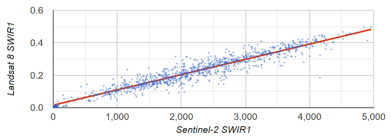
الشكل 2: رسم بياني للنقاط المتفرقة وخط الانحدار الخطي لأصغر مربعات لعيّنة من البكسلات التي تمثّل انعكاس سطح الأرض في نطاقات SWIR1 من بيانات Sentinel-2
وLandsat 8
ee.List
يمكن أن تكون الأعمدة لكائنات ee.List ثنائية الأبعاد مدخلات لأدوات معالجة
الانحدار. تقدّم الأمثلة التالية إثباتات بسيطة؛ فالمتغيّر المستقل هو نسخة من المتغيّر التابع ينتج عنه قيمة ثابتة عند محور y تساوي
0 ومنحدر يساوي 1.
linearFit()
محرِّر الرموز البرمجية (JavaScript)
// Define a list of lists, where columns represent variables. The first column
// is the independent variable and the second is the dependent variable.
var listsVarColumns = ee.List([
  [1, 1],
  [2, 2],
  [3, 3],
  [4, 4],
  [5, 5]
]);

// Compute the least squares estimate of a linear function. Note that an
// object is returned; cast it as an ee.Dictionary to make accessing the
// coefficients easier.
var linearFit = ee.Dictionary(listsVarColumns.reduce(ee.Reducer.linearFit()));

// Inspect the result.
print(linearFit);
print('y-intercept:', linearFit.get('offset'));
print('Slope:', linearFit.get('scale'));
بدِّل صفوف القائمة إلى أعمدة إذا كانت المتغيّرات ممثّلة بصفوف من خلال تحويلها إلى ee.Array، ثم بدِّل صفوفها إلى أعمدة، ثم حوِّلها مرة أخرى إلى ee.List.
محرِّر الرموز البرمجية (JavaScript)
// If variables in the list are arranged as rows, you'll need to transpose it.
// Define a list of lists where rows represent variables. The first row is the
// independent variable and the second is the dependent variable.
var listsVarRows = ee.List([
  [1, 2, 3, 4, 5],
  [1, 2, 3, 4, 5]
]);

// Cast the ee.List as an ee.Array, transpose it, and cast back to ee.List.
var listsVarColumns = ee.Array(listsVarRows).transpose().toList();

// Compute the least squares estimate of a linear function. Note that an
// object is returned; cast it as an ee.Dictionary to make accessing the
// coefficients easier.
var linearFit = ee.Dictionary(listsVarColumns.reduce(ee.Reducer.linearFit()));

// Inspect the result.
print(linearFit);
print('y-intercept:', linearFit.get('offset'));
print('Slope:', linearFit.get('scale'));
linearRegression()
يشبه تطبيق ee.Reducer.linearRegression() مثال linearFit() أعلاه، باستثناء أنّه يتم تضمين متغيّر مستقل ثابت.
محرِّر الرموز البرمجية (JavaScript)
// Define a list of lists where columns represent variables. The first column
// represents a constant term, the second an independent variable, and the third
// a dependent variable.
var listsVarColumns = ee.List([
  [1, 1, 1],
  [1, 2, 2],
  [1, 3, 3],
  [1, 4, 4],
  [1, 5, 5]
]);

// Compute ordinary least squares regression coefficients. numX is 2 because
// there is one constant term and an additional independent variable. numY is 1
// because there is only a single dependent variable. Cast the resulting
// object to an ee.Dictionary for easy access to the properties.
var linearRegression = ee.Dictionary(
  listsVarColumns.reduce(ee.Reducer.linearRegression({
    numX: 2,
    numY: 1
})));

// Convert the coefficients array to a list.
var coefList = ee.Array(linearRegression.get('coefficients')).toList();

// Extract the y-intercept and slope.
var b0 = ee.List(coefList.get(0)).get(0); // y-intercept
var b1 = ee.List(coefList.get(1)).get(0); // slope

// Extract the residuals.
var residuals = ee.Array(linearRegression.get('residuals')).toList().get(0);

// Inspect the results.
print('OLS estimates', linearRegression);
print('y-intercept:', b0);
print('Slope:', b1);
print('Residuals:', residuals);