رگرسیون خطی

Earth Engine چندین روش برای انجام رگرسیون خطی با استفاده از کاهنده ها دارد:

• ee.Reducer.linearFit()
• ee.Reducer.linearRegression()
• ee.Reducer.robustLinearRegression()
• ee.Reducer.ridgeRegression()

ساده ترین کاهنده رگرسیون خطی linearFit() است که برآورد حداقل مربعات یک تابع خطی از یک متغیر را با یک جمله ثابت محاسبه می کند. برای یک رویکرد انعطاف‌پذیرتر به مدل‌سازی خطی، از یکی از کاهنده‌های رگرسیون خطی استفاده کنید که تعداد متغیری از متغیرهای مستقل و وابسته را امکان‌پذیر می‌کند. linearRegression() رگرسیون حداقل مربعات معمولی (OLS) را پیاده سازی می کند. robustLinearRegression() از یک تابع هزینه بر اساس باقیمانده های رگرسیون استفاده می کند تا به طور مکرر وزن های پرت را در داده ها کاهش دهد ( O'Leary, 1990 ). ridgeRegression() رگرسیون خطی را با تنظیم L2 انجام می دهد.

تحلیل رگرسیون با این روش ها برای کاهش اشیاء ee.ImageCollection ، ee.Image ، ee.FeatureCollection و ee.List مناسب است. مثال‌های زیر یک کاربرد را برای هر کدام نشان می‌دهند. توجه داشته باشید که linearRegression() robustLinearRegression() و ridgeRegression() همگی ساختارهای ورودی و خروجی یکسانی دارند، اما linearFit() انتظار دارد ورودی دو بانده ای (X به دنبال Y) و ridgeRegression() دارای یک پارامتر اضافی ( lambda ، اختیاری ) و خروجی ( pValue ) باشد.

توجه: matrixSolve() یک روش جایگزین برای رگرسیون حداقل مربعات ارائه می دهد که به عنوان ee.Reducer پیاده سازی نمی شود.

ee.ImageCollection

linearFit()

داده ها باید به عنوان یک تصویر ورودی دو باندی تنظیم شوند که باند اول متغیر مستقل و باند دوم متغیر وابسته است. مثال زیر تخمین روند خطی بارش آینده (پس از سال 2006 در داده های NEX-DCP30 ) را نشان می دهد که توسط مدل های آب و هوایی پیش بینی شده است. متغیر وابسته بارش پیش بینی شده و متغیر مستقل زمان است که قبل از فراخوانی linearFit() اضافه شده است:

ویرایشگر کد (جاوا اسکریپت)

// This function adds a time band to the image.
var createTimeBand = function(image) {
  // Scale milliseconds by a large constant to avoid very small slopes
  // in the linear regression output.
  return image.addBands(image.metadata('system:time_start').divide(1e18));
};

// Load the input image collection: projected climate data.
var collection = ee.ImageCollection('NASA/NEX-DCP30_ENSEMBLE_STATS')
  .filter(ee.Filter.eq('scenario', 'rcp85'))
  .filterDate(ee.Date('2006-01-01'), ee.Date('2050-01-01'))
  // Map the time band function over the collection.
  .map(createTimeBand);

// Reduce the collection with the linear fit reducer.
// Independent variable are followed by dependent variables.
var linearFit = collection.select(['system:time_start', 'pr_mean'])
  .reduce(ee.Reducer.linearFit());

// Display the results.
Map.setCenter(-100.11, 40.38, 5);
Map.addLayer(linearFit,
  {min: 0, max: [-0.9, 8e-5, 1], bands: ['scale', 'offset', 'scale']}, 'fit');

توجه داشته باشید که خروجی شامل دو باند است، "offset" (برق) و "مقیاس" ("مقیاس" در این زمینه به شیب خط اشاره دارد و نباید با ورودی پارامتر مقیاس به بسیاری از کاهنده ها، که مقیاس فضایی است، اشتباه گرفته شود). نتیجه، با مناطقی با روند افزایشی در آبی، روند کاهشی در قرمز و بدون روند در سبز باید چیزی شبیه به شکل 1 باشد.

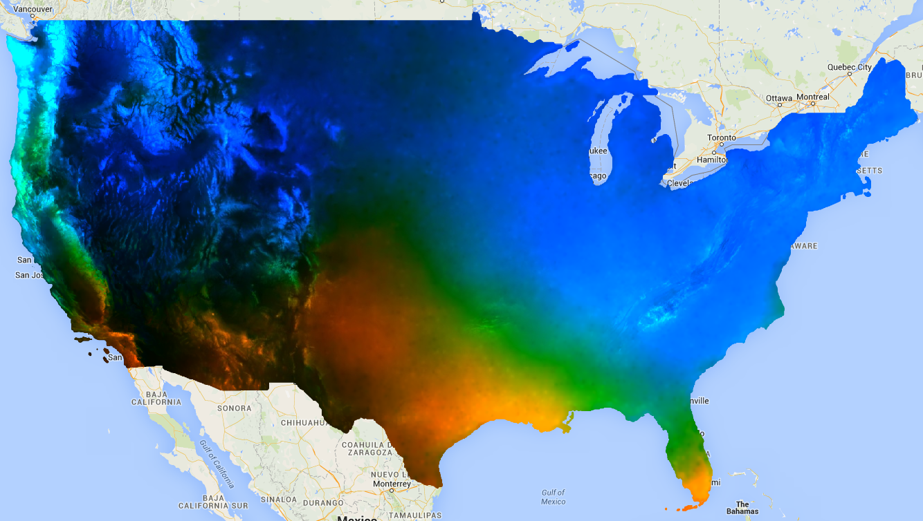
شکل 1. خروجی linearFit() برای بارش پیش بینی شده اعمال می شود. مناطقی که پیش بینی می شود بارش افزایش یابد با رنگ آبی و بارش کاهش یافته با رنگ قرمز نشان داده شده است.

linearRegression()

برای مثال، فرض کنید دو متغیر وابسته وجود دارد: بارش و حداکثر دما، و دو متغیر مستقل: یک ثابت و زمان. مجموعه مشابه مثال قبلی است، اما باند ثابت باید به صورت دستی قبل از کاهش اضافه شود. دو باند اول ورودی، متغیرهای 'X' (مستقل) و دو باند بعدی متغیرهای 'Y' (وابسته) هستند. در این مثال، ابتدا ضرایب رگرسیون را بدست آورید، سپس تصویر آرایه را صاف کنید تا باندهای مورد نظر را استخراج کنید:

ویرایشگر کد (جاوا اسکریپت)

// This function adds a time band to the image.
var createTimeBand = function(image) {
  // Scale milliseconds by a large constant.
  return image.addBands(image.metadata('system:time_start').divide(1e18));
};

// This function adds a constant band to the image.
var createConstantBand = function(image) {
  return ee.Image(1).addBands(image);
};

// Load the input image collection: projected climate data.
var collection = ee.ImageCollection('NASA/NEX-DCP30_ENSEMBLE_STATS')
  .filterDate(ee.Date('2006-01-01'), ee.Date('2099-01-01'))
  .filter(ee.Filter.eq('scenario', 'rcp85'))
  // Map the functions over the collection, to get constant and time bands.
  .map(createTimeBand)
  .map(createConstantBand)
  // Select the predictors and the responses.
  .select(['constant', 'system:time_start', 'pr_mean', 'tasmax_mean']);

// Compute ordinary least squares regression coefficients.
var linearRegression = collection.reduce(
  ee.Reducer.linearRegression({
    numX: 2,
    numY: 2
}));

// Compute robust linear regression coefficients.
var robustLinearRegression = collection.reduce(
  ee.Reducer.robustLinearRegression({
    numX: 2,
    numY: 2
}));

// The results are array images that must be flattened for display.
// These lists label the information along each axis of the arrays.
var bandNames = [['constant', 'time'], // 0-axis variation.
                 ['precip', 'temp']]; // 1-axis variation.

// Flatten the array images to get multi-band images according to the labels.
var lrImage = linearRegression.select(['coefficients']).arrayFlatten(bandNames);
var rlrImage = robustLinearRegression.select(['coefficients']).arrayFlatten(bandNames);

// Display the OLS results.
Map.setCenter(-100.11, 40.38, 5);
Map.addLayer(lrImage,
  {min: 0, max: [-0.9, 8e-5, 1], bands: ['time_precip', 'constant_precip', 'time_precip']}, 'OLS');

// Compare the results at a specific point:
print('OLS estimates:', lrImage.reduceRegion({
  reducer: ee.Reducer.first(),
  geometry: ee.Geometry.Point([-96.0, 41.0]),
  scale: 1000
}));

print('Robust estimates:', rlrImage.reduceRegion({
  reducer: ee.Reducer.first(),
  geometry: ee.Geometry.Point([-96.0, 41.0]),
  scale: 1000
}));

نتایج را بررسی کنید تا متوجه شوید که خروجی linearRegression() معادل ضرایبی است که توسط کاهنده linearFit() تخمین زده شده است، اگرچه خروجی linearRegression() ضرایبی برای متغیر وابسته دیگر، tasmax_mean نیز دارد. ضرایب رگرسیون خطی قوی با تخمین OLS متفاوت است. مثال، ضرایب روش های رگرسیون مختلف را در یک نقطه خاص مقایسه می کند.

ee.تصویر

در زمینه یک شی ee.Image ، کاهنده‌های رگرسیون را می‌توان با reduceRegion یا reduceRegions برای انجام رگرسیون خطی بر روی پیکسل‌ها در ناحیه(ها) استفاده کرد. مثال‌های زیر نحوه محاسبه ضرایب رگرسیون بین باندهای Landsat را در یک چندضلعی دلخواه نشان می‌دهند.

linearFit()

بخش راهنما که نمودارهای داده‌های آرایه را توصیف می‌کند، نمودار پراکندگی همبستگی بین باندهای Landsat 8 SWIR1 و SWIR2 را نشان می‌دهد. در اینجا ضرایب رگرسیون خطی برای این رابطه محاسبه می شود. فرهنگ لغت حاوی ویژگی های 'offset' (y-intercept) و 'scale' (slope) برگردانده می شود.

ویرایشگر کد (جاوا اسکریپت)

// Define a rectangle geometry around San Francisco.
var sanFrancisco = ee.Geometry.Rectangle([-122.45, 37.74, -122.4, 37.8]);

// Import a Landsat 8 TOA image for this region.
var img = ee.Image('LANDSAT/LC08/C02/T1_TOA/LC08_044034_20140318');

// Subset the SWIR1 and SWIR2 bands. In the regression reducer, independent
// variables come first followed by the dependent variables. In this case,
// B5 (SWIR1) is the independent variable and B6 (SWIR2) is the dependent
// variable.
var imgRegress = img.select(['B5', 'B6']);

// Calculate regression coefficients for the set of pixels intersecting the
// above defined region using reduceRegion with ee.Reducer.linearFit().
var linearFit = imgRegress.reduceRegion({
  reducer: ee.Reducer.linearFit(),
  geometry: sanFrancisco,
  scale: 30,
});

// Inspect the results.
print('OLS estimates:', linearFit);
print('y-intercept:', linearFit.get('offset'));
print('Slope:', linearFit.get('scale'));

linearRegression()

همان تجزیه و تحلیل از بخش linearFit قبلی در اینجا اعمال می شود، با این تفاوت که این بار از تابع ee.Reducer.linearRegression استفاده می شود. توجه داشته باشید که یک تصویر رگرسیون از سه تصویر مجزا ساخته می‌شود: یک تصویر ثابت و تصاویری که نوارهای SWIR1 و SWIR2 را از همان تصویر Landsat 8 نشان می‌دهند. به خاطر داشته باشید که می توانید هر مجموعه ای از باندها را ترکیب کنید تا یک تصویر ورودی برای کاهش ناحیه توسط ee.Reducer.linearRegression بسازید، لازم نیست آنها به یک تصویر منبع تعلق داشته باشند.

ویرایشگر کد (جاوا اسکریپت)

// Define a rectangle geometry around San Francisco.
var sanFrancisco = ee.Geometry.Rectangle([-122.45, 37.74, -122.4, 37.8]);

// Import a Landsat 8 TOA image for this region.
var img = ee.Image('LANDSAT/LC08/C02/T1_TOA/LC08_044034_20140318');

// Create a new image that is the concatenation of three images: a constant,
// the SWIR1 band, and the SWIR2 band.
var constant = ee.Image(1);
var xVar = img.select('B5');
var yVar = img.select('B6');
var imgRegress = ee.Image.cat(constant, xVar, yVar);

// Calculate regression coefficients for the set of pixels intersecting the
// above defined region using reduceRegion. The numX parameter is set as 2
// because the constant and the SWIR1 bands are independent variables and they
// are the first two bands in the stack; numY is set as 1 because there is only
// one dependent variable (SWIR2) and it follows as band three in the stack.
var linearRegression = imgRegress.reduceRegion({
  reducer: ee.Reducer.linearRegression({
    numX: 2,
    numY: 1
  }),
  geometry: sanFrancisco,
  scale: 30,
});

// Convert the coefficients array to a list.
var coefList = ee.Array(linearRegression.get('coefficients')).toList();

// Extract the y-intercept and slope.
var b0 = ee.List(coefList.get(0)).get(0); // y-intercept
var b1 = ee.List(coefList.get(1)).get(0); // slope

// Extract the residuals.
var residuals = ee.Array(linearRegression.get('residuals')).toList().get(0);

// Inspect the results.
print('OLS estimates', linearRegression);
print('y-intercept:', b0);
print('Slope:', b1);
print('Residuals:', residuals);

فرهنگ لغت حاوی ویژگی های 'coefficients' و 'residuals' برگردانده می شود. ویژگی 'coefficients' آرایه ای با ابعاد (numX, numY) است. هر ستون شامل ضرایب متغیر وابسته مربوطه است. در این حالت، آرایه دارای دو سطر و یک ستون است. سطر یک، ستون یک خط y و سطر دو، ستون یک شیب است. ویژگی 'residuals' بردار ریشه میانگین مربع باقیمانده های هر متغیر وابسته است. ضرایب را با ریختن نتیجه به عنوان یک آرایه و سپس برش دادن عناصر مورد نظر یا تبدیل آرایه به لیست و انتخاب ضرایب بر اساس موقعیت شاخص استخراج کنید.

ee.FeatureCollection

فرض کنید می خواهید رابطه خطی بین بازتاب Sentinel-2 و Landsat 8 SWIR1 را بدانید. در این مثال، یک نمونه تصادفی از پیکسل‌هایی که به‌عنوان مجموعه ویژگی‌هایی از نقاط قالب‌بندی شده‌اند برای محاسبه رابطه استفاده می‌شوند. یک نمودار پراکندگی از جفت پیکسل ها به همراه خط کمترین مربع با بهترین تناسب تولید می شود (شکل 2).

ویرایشگر کد (جاوا اسکریپت)

// Import a Sentinel-2 TOA image.
var s2ImgSwir1 = ee.Image('COPERNICUS/S2/20191022T185429_20191022T185427_T10SEH');

// Import a Landsat 8 TOA image from 12 days earlier than the S2 image.
var l8ImgSwir1 = ee.Image('LANDSAT/LC08/C02/T1_TOA/LC08_044033_20191010');

// Get the intersection between the two images - the area of interest (aoi).
var aoi = s2ImgSwir1.geometry().intersection(l8ImgSwir1.geometry());

// Get a set of 1000 random points from within the aoi. A feature collection
// is returned.
var sample = ee.FeatureCollection.randomPoints({
  region: aoi,
  points: 1000
});

// Combine the SWIR1 bands from each image into a single image.
var swir1Bands = s2ImgSwir1.select('B11')
  .addBands(l8ImgSwir1.select('B6'))
  .rename(['s2_swir1', 'l8_swir1']);

// Sample the SWIR1 bands using the sample point feature collection.
var imgSamp = swir1Bands.sampleRegions({
  collection: sample,
  scale: 30
})
// Add a constant property to each feature to be used as an independent variable.
.map(function(feature) {
  return feature.set('constant', 1);
});

// Compute linear regression coefficients. numX is 2 because
// there are two independent variables: 'constant' and 's2_swir1'. numY is 1
// because there is a single dependent variable: 'l8_swir1'. Cast the resulting
// object to an ee.Dictionary for easy access to the properties.
var linearRegression = ee.Dictionary(imgSamp.reduceColumns({
  reducer: ee.Reducer.linearRegression({
    numX: 2,
    numY: 1
  }),
  selectors: ['constant', 's2_swir1', 'l8_swir1']
}));

// Convert the coefficients array to a list.
var coefList = ee.Array(linearRegression.get('coefficients')).toList();

// Extract the y-intercept and slope.
var yInt = ee.List(coefList.get(0)).get(0); // y-intercept
var slope = ee.List(coefList.get(1)).get(0); // slope

// Gather the SWIR1 values from the point sample into a list of lists.
var props = ee.List(['s2_swir1', 'l8_swir1']);
var regressionVarsList = ee.List(imgSamp.reduceColumns({
  reducer: ee.Reducer.toList().repeat(props.size()),
  selectors: props
}).get('list'));

// Convert regression x and y variable lists to an array - used later as input
// to ui.Chart.array.values for generating a scatter plot.
var x = ee.Array(ee.List(regressionVarsList.get(0)));
var y1 = ee.Array(ee.List(regressionVarsList.get(1)));

// Apply the line function defined by the slope and y-intercept of the
// regression to the x variable list to create an array that will represent
// the regression line in the scatter plot.
var y2 = ee.Array(ee.List(regressionVarsList.get(0)).map(function(x) {
  var y = ee.Number(x).multiply(slope).add(yInt);
  return y;
}));

// Concatenate the y variables (Landsat 8 SWIR1 and predicted y) into an array
// for input to ui.Chart.array.values for plotting a scatter plot.
var yArr = ee.Array.cat([y1, y2], 1);

// Make a scatter plot of the two SWIR1 bands for the point sample and include
// the least squares line of best fit through the data.
print(ui.Chart.array.values({
  array: yArr,
  axis: 0,
  xLabels: x})
  .setChartType('ScatterChart')
  .setOptions({
    legend: {position: 'none'},
    hAxis: {'title': 'Sentinel-2 SWIR1'},
    vAxis: {'title': 'Landsat 8 SWIR1'},
    series: {
      0: {
        pointSize: 0.2,
        dataOpacity: 0.5,
      },
      1: {
        pointSize: 0,
        lineWidth: 2,
      }
    }
  })
);

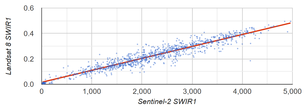
شکل 2. نمودار پراکندگی و خط رگرسیون خطی حداقل مربعات برای نمونه ای از پیکسل های نشان دهنده بازتاب Sentinel-2 و Landsat 8 SWIR1 TOA.

ee.List

ستون های 2-D اشیاء ee.List می توانند ورودی برای کاهش دهنده های رگرسیون باشند. مثال‌های زیر شواهد ساده‌ای را ارائه می‌کنند. متغیر مستقل یک کپی از متغیر وابسته است که یک تقاطع y برابر با 0 و یک شیب برابر با 1 ایجاد می کند.

توجه: که نتیجه کاهش ee.List یک شی است. آن را به ee.Dictionary ارسال کنید تا دسترسی به ویژگی ها آسان تر شود.

احتیاط: طول بین سطرها و ستون ها باید برابر باشد. از null برای نشان دادن ورودی های داده از دست رفته استفاده کنید.

linearFit()

ویرایشگر کد (جاوا اسکریپت)

// Define a list of lists, where columns represent variables. The first column
// is the independent variable and the second is the dependent variable.
var listsVarColumns = ee.List([
  [1, 1],
  [2, 2],
  [3, 3],
  [4, 4],
  [5, 5]
]);

// Compute the least squares estimate of a linear function. Note that an
// object is returned; cast it as an ee.Dictionary to make accessing the
// coefficients easier.
var linearFit = ee.Dictionary(listsVarColumns.reduce(ee.Reducer.linearFit()));

// Inspect the result.
print(linearFit);
print('y-intercept:', linearFit.get('offset'));
print('Slope:', linearFit.get('scale'));

اگر متغیرها با ردیف‌هایی با تبدیل به ee.Array ، جابجایی آن و سپس تبدیل مجدد به ee.List ، فهرست را جابه‌جا کنید .

ویرایشگر کد (جاوا اسکریپت)

// If variables in the list are arranged as rows, you'll need to transpose it.
// Define a list of lists where rows represent variables. The first row is the
// independent variable and the second is the dependent variable.
var listsVarRows = ee.List([
  [1, 2, 3, 4, 5],
  [1, 2, 3, 4, 5]
]);

// Cast the ee.List as an ee.Array, transpose it, and cast back to ee.List.
var listsVarColumns = ee.Array(listsVarRows).transpose().toList();

// Compute the least squares estimate of a linear function. Note that an
// object is returned; cast it as an ee.Dictionary to make accessing the
// coefficients easier.
var linearFit = ee.Dictionary(listsVarColumns.reduce(ee.Reducer.linearFit()));

// Inspect the result.
print(linearFit);
print('y-intercept:', linearFit.get('offset'));
print('Slope:', linearFit.get('scale'));

linearRegression()

کاربرد ee.Reducer.linearRegression() مشابه مثال linearFit() فوق است، با این تفاوت که یک متغیر مستقل ثابت گنجانده شده است.

ویرایشگر کد (جاوا اسکریپت)

// Define a list of lists where columns represent variables. The first column
// represents a constant term, the second an independent variable, and the third
// a dependent variable.
var listsVarColumns = ee.List([
  [1, 1, 1],
  [1, 2, 2],
  [1, 3, 3],
  [1, 4, 4],
  [1, 5, 5]
]);

// Compute ordinary least squares regression coefficients. numX is 2 because
// there is one constant term and an additional independent variable. numY is 1
// because there is only a single dependent variable. Cast the resulting
// object to an ee.Dictionary for easy access to the properties.
var linearRegression = ee.Dictionary(
  listsVarColumns.reduce(ee.Reducer.linearRegression({
    numX: 2,
    numY: 1
})));

// Convert the coefficients array to a list.
var coefList = ee.Array(linearRegression.get('coefficients')).toList();

// Extract the y-intercept and slope.
var b0 = ee.List(coefList.get(0)).get(0); // y-intercept
var b1 = ee.List(coefList.get(1)).get(0); // slope

// Extract the residuals.
var residuals = ee.Array(linearRegression.get('residuals')).toList().get(0);

// Inspect the results.
print('OLS estimates', linearRegression);
print('y-intercept:', b0);
print('Slope:', b1);
print('Residuals:', residuals);