Regresi Linear

Earth Engine memiliki beberapa metode untuk melakukan regresi linear menggunakan pengurangan:

• ee.Reducer.linearFit()
• ee.Reducer.linearRegression()
• ee.Reducer.robustLinearRegression()
• ee.Reducer.ridgeRegression()

Pengurang regresi linear yang paling sederhana adalah linearFit() yang menghitung estimasi kuadrat terkecil dari fungsi linear satu variabel dengan istilah konstan. Untuk pendekatan yang lebih fleksibel dalam pemodelan linear, gunakan salah satu pengurang regresi linear yang memungkinkan jumlah variabel independen dan dependen yang bervariasi. linearRegression() menerapkan regresi kuadrat terkecil biasa(OLS). robustLinearRegression() menggunakan fungsi biaya berdasarkan residu regresi untuk mengurangi bobot outlier secara iteratif dalam data (O'Leary, 1990). ridgeRegression() melakukan regresi linear dengan regularisasi L2.

Analisis regresi dengan metode ini cocok untuk mengurangi objek ee.ImageCollection, ee.Image, ee.FeatureCollection, dan ee.List. Contoh berikut menunjukkan aplikasi untuk setiap jenis. Perhatikan bahwa linearRegression(), robustLinearRegression(), dan ridgeRegression() semuanya memiliki struktur input dan output yang sama, tetapi linearFit() mengharapkan input dua band (X diikuti dengan Y) dan ridgeRegression() memiliki parameter tambahan (lambda, opsional) dan output (pValue).

Catatan: matrixSolve() menyediakan metode alternatif untuk regresi kuadrat terkecil yang tidak diterapkan sebagai ee.Reducer.

ee.ImageCollection

linearFit()

Data harus disiapkan sebagai gambar input dua band, dengan band pertama adalah variabel independen dan band kedua adalah variabel dependen. Contoh berikut menunjukkan estimasi tren linear presipitasi mendatang (setelah 2006 dalam data NEX-DCP30) yang diproyeksikan oleh model iklim. Variabel dependen adalah proyeksi presipitasi dan variabel independen adalah waktu, yang ditambahkan sebelum memanggil linearFit():

Editor Kode (JavaScript)

// This function adds a time band to the image.
var createTimeBand = function(image) {
  // Scale milliseconds by a large constant to avoid very small slopes
  // in the linear regression output.
  return image.addBands(image.metadata('system:time_start').divide(1e18));
};

// Load the input image collection: projected climate data.
var collection = ee.ImageCollection('NASA/NEX-DCP30_ENSEMBLE_STATS')
  .filter(ee.Filter.eq('scenario', 'rcp85'))
  .filterDate(ee.Date('2006-01-01'), ee.Date('2050-01-01'))
  // Map the time band function over the collection.
  .map(createTimeBand);

// Reduce the collection with the linear fit reducer.
// Independent variable are followed by dependent variables.
var linearFit = collection.select(['system:time_start', 'pr_mean'])
  .reduce(ee.Reducer.linearFit());

// Display the results.
Map.setCenter(-100.11, 40.38, 5);
Map.addLayer(linearFit,
  {min: 0, max: [-0.9, 8e-5, 1], bands: ['scale', 'offset', 'scale']}, 'fit');

Perhatikan bahwa output berisi dua band, 'offset' (intersep) dan 'skala' ('skala' dalam konteks ini mengacu pada kemiringan garis dan tidak harus disamakan dengan input parameter skala ke banyak pengurangan, yang merupakan skala spasial). Hasilnya, dengan area tren meningkat berwarna biru, tren menurun berwarna merah, dan tidak ada tren berwarna hijau akan terlihat seperti Gambar 1.

Gambar 1. Output linearFit() diterapkan ke proyeksi presipitasi. Area yang diproyeksikan akan mengalami peningkatan presipitasi ditampilkan dalam warna biru dan presipitasi yang menurun dalam warna merah.

linearRegression()

Misalnya, ada dua variabel dependen: presipitasi dan suhu maksimum, serta dua variabel independen: konstanta dan waktu. Koleksi ini identik dengan contoh sebelumnya, tetapi band konstan harus ditambahkan secara manual sebelum pengurangan. Dua band pertama input adalah variabel 'X' (independen) dan dua band berikutnya adalah variabel 'Y' (dependen). Dalam contoh ini, pertama-tama dapatkan koefisien regresi, lalu ratakan gambar array untuk mengekstrak band yang diinginkan:

Editor Kode (JavaScript)

// This function adds a time band to the image.
var createTimeBand = function(image) {
  // Scale milliseconds by a large constant.
  return image.addBands(image.metadata('system:time_start').divide(1e18));
};

// This function adds a constant band to the image.
var createConstantBand = function(image) {
  return ee.Image(1).addBands(image);
};

// Load the input image collection: projected climate data.
var collection = ee.ImageCollection('NASA/NEX-DCP30_ENSEMBLE_STATS')
  .filterDate(ee.Date('2006-01-01'), ee.Date('2099-01-01'))
  .filter(ee.Filter.eq('scenario', 'rcp85'))
  // Map the functions over the collection, to get constant and time bands.
  .map(createTimeBand)
  .map(createConstantBand)
  // Select the predictors and the responses.
  .select(['constant', 'system:time_start', 'pr_mean', 'tasmax_mean']);

// Compute ordinary least squares regression coefficients.
var linearRegression = collection.reduce(
  ee.Reducer.linearRegression({
    numX: 2,
    numY: 2
}));

// Compute robust linear regression coefficients.
var robustLinearRegression = collection.reduce(
  ee.Reducer.robustLinearRegression({
    numX: 2,
    numY: 2
}));

// The results are array images that must be flattened for display.
// These lists label the information along each axis of the arrays.
var bandNames = [['constant', 'time'], // 0-axis variation.
                 ['precip', 'temp']]; // 1-axis variation.

// Flatten the array images to get multi-band images according to the labels.
var lrImage = linearRegression.select(['coefficients']).arrayFlatten(bandNames);
var rlrImage = robustLinearRegression.select(['coefficients']).arrayFlatten(bandNames);

// Display the OLS results.
Map.setCenter(-100.11, 40.38, 5);
Map.addLayer(lrImage,
  {min: 0, max: [-0.9, 8e-5, 1], bands: ['time_precip', 'constant_precip', 'time_precip']}, 'OLS');

// Compare the results at a specific point:
print('OLS estimates:', lrImage.reduceRegion({
  reducer: ee.Reducer.first(),
  geometry: ee.Geometry.Point([-96.0, 41.0]),
  scale: 1000
}));

print('Robust estimates:', rlrImage.reduceRegion({
  reducer: ee.Reducer.first(),
  geometry: ee.Geometry.Point([-96.0, 41.0]),
  scale: 1000
}));

Periksa hasilnya untuk menemukan bahwa output linearRegression() setara dengan koefisien yang diperkirakan oleh pengurangan linearFit(), meskipun output linearRegression() juga memiliki koefisien untuk variabel dependen lainnya, tasmax_mean. Koefisien regresi linear yang andal berbeda dengan estimasi OLS. Contoh ini membandingkan koefisien dari metode regresi yang berbeda pada titik tertentu.

ee.Image

Dalam konteks objek ee.Image, pengurangan regresi dapat digunakan dengan reduceRegion atau reduceRegions untuk melakukan regresi linear pada piksel di region. Contoh berikut menunjukkan cara menghitung koefisien regresi antara band Landsat dalam poligon arbitrer.

linearFit()

Bagian panduan yang menjelaskan diagram data array menampilkan plot pencar korelasi antara band SWIR1 dan SWIR2 Landsat 8. Di sini, koefisien regresi linear untuk hubungan ini dihitung. Kamus yang berisi properti 'offset' (titik perpotongan y) dan 'scale' (kemiringan) akan ditampilkan.

Editor Kode (JavaScript)

// Define a rectangle geometry around San Francisco.
var sanFrancisco = ee.Geometry.Rectangle([-122.45, 37.74, -122.4, 37.8]);

// Import a Landsat 8 TOA image for this region.
var img = ee.Image('LANDSAT/LC08/C02/T1_TOA/LC08_044034_20140318');

// Subset the SWIR1 and SWIR2 bands. In the regression reducer, independent
// variables come first followed by the dependent variables. In this case,
// B5 (SWIR1) is the independent variable and B6 (SWIR2) is the dependent
// variable.
var imgRegress = img.select(['B5', 'B6']);

// Calculate regression coefficients for the set of pixels intersecting the
// above defined region using reduceRegion with ee.Reducer.linearFit().
var linearFit = imgRegress.reduceRegion({
  reducer: ee.Reducer.linearFit(),
  geometry: sanFrancisco,
  scale: 30,
});

// Inspect the results.
print('OLS estimates:', linearFit);
print('y-intercept:', linearFit.get('offset'));
print('Slope:', linearFit.get('scale'));

linearRegression()

Analisis yang sama dari bagian linearFit sebelumnya diterapkan di sini, kecuali kali ini fungsi ee.Reducer.linearRegression digunakan. Perhatikan bahwa gambar regresi dibuat dari tiga gambar terpisah: gambar konstan dan gambar yang mewakili band SWIR1 dan SWIR2 dari gambar Landsat 8 yang sama. Perlu diingat bahwa Anda dapat menggabungkan kumpulan band apa pun untuk membuat gambar input untuk pengurangan wilayah dengan ee.Reducer.linearRegression, kumpulan band tersebut tidak harus merupakan bagian dari gambar sumber yang sama.

Editor Kode (JavaScript)

// Define a rectangle geometry around San Francisco.
var sanFrancisco = ee.Geometry.Rectangle([-122.45, 37.74, -122.4, 37.8]);

// Import a Landsat 8 TOA image for this region.
var img = ee.Image('LANDSAT/LC08/C02/T1_TOA/LC08_044034_20140318');

// Create a new image that is the concatenation of three images: a constant,
// the SWIR1 band, and the SWIR2 band.
var constant = ee.Image(1);
var xVar = img.select('B5');
var yVar = img.select('B6');
var imgRegress = ee.Image.cat(constant, xVar, yVar);

// Calculate regression coefficients for the set of pixels intersecting the
// above defined region using reduceRegion. The numX parameter is set as 2
// because the constant and the SWIR1 bands are independent variables and they
// are the first two bands in the stack; numY is set as 1 because there is only
// one dependent variable (SWIR2) and it follows as band three in the stack.
var linearRegression = imgRegress.reduceRegion({
  reducer: ee.Reducer.linearRegression({
    numX: 2,
    numY: 1
  }),
  geometry: sanFrancisco,
  scale: 30,
});

// Convert the coefficients array to a list.
var coefList = ee.Array(linearRegression.get('coefficients')).toList();

// Extract the y-intercept and slope.
var b0 = ee.List(coefList.get(0)).get(0); // y-intercept
var b1 = ee.List(coefList.get(1)).get(0); // slope

// Extract the residuals.
var residuals = ee.Array(linearRegression.get('residuals')).toList().get(0);

// Inspect the results.
print('OLS estimates', linearRegression);
print('y-intercept:', b0);
print('Slope:', b1);
print('Residuals:', residuals);

Kamus yang berisi properti 'coefficients' dan 'residuals' akan ditampilkan. Properti 'coefficients' adalah array dengan dimensi (numX, numY); setiap kolom berisi koefisien untuk variabel dependen yang sesuai. Dalam hal ini, array memiliki dua baris dan satu kolom; baris satu, kolom satu adalah intersep y dan baris dua, kolom satu adalah kemiringan. Properti 'residuals' adalah vektor root mean square dari residu setiap variabel dependen. Ekstrak koefisien dengan mentransmisikan hasilnya sebagai array, lalu memotong elemen yang diinginkan atau mengonversi array menjadi daftar dan memilih koefisien menurut posisi indeks.

ee.FeatureCollection

Misalkan Anda ingin mengetahui hubungan linear antara Sentinel-2 dan reflektansi SWIR1 Landsat 8. Dalam contoh ini, sampel acak piksel yang diformat sebagai kumpulan fitur titik digunakan untuk menghitung hubungan. Plot pencar pasangan piksel beserta garis least squares yang paling sesuai akan dihasilkan (Gambar 2).

Editor Kode (JavaScript)

// Import a Sentinel-2 TOA image.
var s2ImgSwir1 = ee.Image('COPERNICUS/S2/20191022T185429_20191022T185427_T10SEH');

// Import a Landsat 8 TOA image from 12 days earlier than the S2 image.
var l8ImgSwir1 = ee.Image('LANDSAT/LC08/C02/T1_TOA/LC08_044033_20191010');

// Get the intersection between the two images - the area of interest (aoi).
var aoi = s2ImgSwir1.geometry().intersection(l8ImgSwir1.geometry());

// Get a set of 1000 random points from within the aoi. A feature collection
// is returned.
var sample = ee.FeatureCollection.randomPoints({
  region: aoi,
  points: 1000
});

// Combine the SWIR1 bands from each image into a single image.
var swir1Bands = s2ImgSwir1.select('B11')
  .addBands(l8ImgSwir1.select('B6'))
  .rename(['s2_swir1', 'l8_swir1']);

// Sample the SWIR1 bands using the sample point feature collection.
var imgSamp = swir1Bands.sampleRegions({
  collection: sample,
  scale: 30
})
// Add a constant property to each feature to be used as an independent variable.
.map(function(feature) {
  return feature.set('constant', 1);
});

// Compute linear regression coefficients. numX is 2 because
// there are two independent variables: 'constant' and 's2_swir1'. numY is 1
// because there is a single dependent variable: 'l8_swir1'. Cast the resulting
// object to an ee.Dictionary for easy access to the properties.
var linearRegression = ee.Dictionary(imgSamp.reduceColumns({
  reducer: ee.Reducer.linearRegression({
    numX: 2,
    numY: 1
  }),
  selectors: ['constant', 's2_swir1', 'l8_swir1']
}));

// Convert the coefficients array to a list.
var coefList = ee.Array(linearRegression.get('coefficients')).toList();

// Extract the y-intercept and slope.
var yInt = ee.List(coefList.get(0)).get(0); // y-intercept
var slope = ee.List(coefList.get(1)).get(0); // slope

// Gather the SWIR1 values from the point sample into a list of lists.
var props = ee.List(['s2_swir1', 'l8_swir1']);
var regressionVarsList = ee.List(imgSamp.reduceColumns({
  reducer: ee.Reducer.toList().repeat(props.size()),
  selectors: props
}).get('list'));

// Convert regression x and y variable lists to an array - used later as input
// to ui.Chart.array.values for generating a scatter plot.
var x = ee.Array(ee.List(regressionVarsList.get(0)));
var y1 = ee.Array(ee.List(regressionVarsList.get(1)));

// Apply the line function defined by the slope and y-intercept of the
// regression to the x variable list to create an array that will represent
// the regression line in the scatter plot.
var y2 = ee.Array(ee.List(regressionVarsList.get(0)).map(function(x) {
  var y = ee.Number(x).multiply(slope).add(yInt);
  return y;
}));

// Concatenate the y variables (Landsat 8 SWIR1 and predicted y) into an array
// for input to ui.Chart.array.values for plotting a scatter plot.
var yArr = ee.Array.cat([y1, y2], 1);

// Make a scatter plot of the two SWIR1 bands for the point sample and include
// the least squares line of best fit through the data.
print(ui.Chart.array.values({
  array: yArr,
  axis: 0,
  xLabels: x})
  .setChartType('ScatterChart')
  .setOptions({
    legend: {position: 'none'},
    hAxis: {'title': 'Sentinel-2 SWIR1'},
    vAxis: {'title': 'Landsat 8 SWIR1'},
    series: {
      0: {
        pointSize: 0.2,
        dataOpacity: 0.5,
      },
      1: {
        pointSize: 0,
        lineWidth: 2,
      }
    }
  })
);

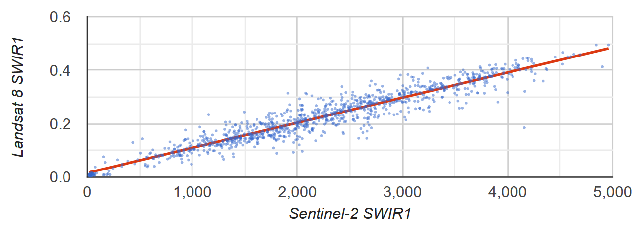
Gambar 2. Diagram pencar dan garis regresi linear kuadrat terkecil untuk sampel piksel yang mewakili pantulan TOA SWIR1 Sentinel-2 dan Landsat 8.

ee.List

Kolom objek ee.List 2D dapat menjadi input untuk pengurangan regresi. Contoh berikut memberikan bukti sederhana; variabel independen adalah salinan variabel dependen yang menghasilkan titik singgung y sama dengan 0 dan kemiringan sama dengan 1.

Catatan: bahwa hasil pengurangan ee.List adalah objek. Transmisikan ke ee.Dictionary untuk mempermudah akses properti.

Perhatian: panjang di antara baris dan kolom harus sama. Gunakan null untuk mewakili entri data yang hilang.

linearFit()

Editor Kode (JavaScript)

// Define a list of lists, where columns represent variables. The first column
// is the independent variable and the second is the dependent variable.
var listsVarColumns = ee.List([
  [1, 1],
  [2, 2],
  [3, 3],
  [4, 4],
  [5, 5]
]);

// Compute the least squares estimate of a linear function. Note that an
// object is returned; cast it as an ee.Dictionary to make accessing the
// coefficients easier.
var linearFit = ee.Dictionary(listsVarColumns.reduce(ee.Reducer.linearFit()));

// Inspect the result.
print(linearFit);
print('y-intercept:', linearFit.get('offset'));
print('Slope:', linearFit.get('scale'));

Transpon daftar jika variabel direpresentasikan oleh baris dengan mengonversi ke ee.Array, mentransponnya, lalu mengonversi kembali ke ee.List.

Editor Kode (JavaScript)

// If variables in the list are arranged as rows, you'll need to transpose it.
// Define a list of lists where rows represent variables. The first row is the
// independent variable and the second is the dependent variable.
var listsVarRows = ee.List([
  [1, 2, 3, 4, 5],
  [1, 2, 3, 4, 5]
]);

// Cast the ee.List as an ee.Array, transpose it, and cast back to ee.List.
var listsVarColumns = ee.Array(listsVarRows).transpose().toList();

// Compute the least squares estimate of a linear function. Note that an
// object is returned; cast it as an ee.Dictionary to make accessing the
// coefficients easier.
var linearFit = ee.Dictionary(listsVarColumns.reduce(ee.Reducer.linearFit()));

// Inspect the result.
print(linearFit);
print('y-intercept:', linearFit.get('offset'));
print('Slope:', linearFit.get('scale'));

linearRegression()

Penerapan ee.Reducer.linearRegression() mirip dengan contoh linearFit() di atas, kecuali bahwa variabel independen konstan disertakan.

Editor Kode (JavaScript)

// Define a list of lists where columns represent variables. The first column
// represents a constant term, the second an independent variable, and the third
// a dependent variable.
var listsVarColumns = ee.List([
  [1, 1, 1],
  [1, 2, 2],
  [1, 3, 3],
  [1, 4, 4],
  [1, 5, 5]
]);

// Compute ordinary least squares regression coefficients. numX is 2 because
// there is one constant term and an additional independent variable. numY is 1
// because there is only a single dependent variable. Cast the resulting
// object to an ee.Dictionary for easy access to the properties.
var linearRegression = ee.Dictionary(
  listsVarColumns.reduce(ee.Reducer.linearRegression({
    numX: 2,
    numY: 1
})));

// Convert the coefficients array to a list.
var coefList = ee.Array(linearRegression.get('coefficients')).toList();

// Extract the y-intercept and slope.
var b0 = ee.List(coefList.get(0)).get(0); // y-intercept
var b1 = ee.List(coefList.get(1)).get(0); // slope

// Extract the residuals.
var residuals = ee.Array(linearRegression.get('residuals')).toList().get(0);

// Inspect the results.
print('OLS estimates', linearRegression);
print('y-intercept:', b0);
print('Slope:', b1);
print('Residuals:', residuals);