Earth Engine có một số phương thức để thực hiện hồi quy tuyến tính bằng cách sử dụng trình giảm:
ee.Reducer.linearFit()ee.Reducer.linearRegression()ee.Reducer.robustLinearRegression()ee.Reducer.ridgeRegression()
Bộ giảm hồi quy tuyến tính đơn giản nhất là linearFit(). Bộ giảm này tính toán ước tính bình phương tối thiểu của một hàm tuyến tính của một biến có một hằng số. Để có phương pháp linh hoạt hơn trong việc lập mô hình tuyến tính, hãy sử dụng một trong các trình giảm hồi quy tuyến tính cho phép số lượng biến độc lập và biến phụ thuộc thay đổi. linearRegression() triển khai hồi quy bình phương tối thiểu thông thường(OLS). robustLinearRegression() sử dụng hàm chi phí dựa trên phần dư hồi quy để lặp lại việc giảm trọng số cho các giá trị ngoại lai trong dữ liệu (O’Leary, 1990).
ridgeRegression() thực hiện hồi quy tuyến tính với quy trình điều hoà L2.
Phân tích hồi quy bằng các phương thức này phù hợp để giảm đối tượng ee.ImageCollection, ee.Image, ee.FeatureCollection và ee.List.
Các ví dụ sau đây minh hoạ cách áp dụng cho từng loại. Xin lưu ý rằng linearRegression(), robustLinearRegression() và ridgeRegression() đều có cùng cấu trúc đầu vào và đầu ra, nhưng linearFit() dự kiến đầu vào hai băng tần (X theo sau là Y) và ridgeRegression() có một tham số bổ sung (lambda, không bắt buộc) và đầu ra (pValue).
ee.ImageCollection
linearFit()
Bạn nên thiết lập dữ liệu dưới dạng hình ảnh đầu vào hai băng, trong đó băng đầu tiên là biến độc lập và băng thứ hai là biến phụ thuộc. Ví dụ sau đây cho thấy kết quả ước tính xu hướng tuyến tính của lượng mưa trong tương lai (sau năm 2006 trong dữ liệu NEX-DCP30) do các mô hình khí hậu dự báo. Biến phụ thuộc là lượng mưa dự kiến và biến độc lập là thời gian, được thêm vào trước khi gọi linearFit():
Trình soạn thảo mã (JavaScript)
// This function adds a time band to the image.
var createTimeBand = function(image) {
  // Scale milliseconds by a large constant to avoid very small slopes
  // in the linear regression output.
  return image.addBands(image.metadata('system:time_start').divide(1e18));
};

// Load the input image collection: projected climate data.
var collection = ee.ImageCollection('NASA/NEX-DCP30_ENSEMBLE_STATS')
  .filter(ee.Filter.eq('scenario', 'rcp85'))
  .filterDate(ee.Date('2006-01-01'), ee.Date('2050-01-01'))
  // Map the time band function over the collection.
  .map(createTimeBand);

// Reduce the collection with the linear fit reducer.
// Independent variable are followed by dependent variables.
var linearFit = collection.select(['system:time_start', 'pr_mean'])
  .reduce(ee.Reducer.linearFit());

// Display the results.
Map.setCenter(-100.11, 40.38, 5);
Map.addLayer(linearFit,
  {min: 0, max: [-0.9, 8e-5, 1], bands: ['scale', 'offset', 'scale']}, 'fit');
Hãy quan sát kết quả chứa hai dải, "offset" (giá trị chênh lệch) và "scale" (tỷ lệ). "Scale" trong ngữ cảnh này đề cập đến độ dốc của đường và không được nhầm lẫn với tham số tỷ lệ đầu vào cho nhiều bộ giảm, tức là tỷ lệ không gian). Kết quả, với các khu vực có xu hướng tăng màu xanh dương, xu hướng giảm màu đỏ và không có xu hướng màu xanh lục sẽ có dạng như Hình 1.

Hình 1. Kết quả của linearFit() được áp dụng cho lượng mưa dự kiến. Những khu vực dự kiến sẽ có lượng mưa tăng lên sẽ hiển thị màu xanh dương và những khu vực dự kiến sẽ có lượng mưa giảm sẽ hiển thị màu đỏ.
linearRegression()
Ví dụ: giả sử có hai biến phụ thuộc: lượng mưa và nhiệt độ tối đa, cùng hai biến độc lập: hằng số và thời gian. Tập hợp này giống hệt với ví dụ trước, nhưng bạn phải thêm dải hằng số theo cách thủ công trước khi giảm. Hai dải đầu tiên của dữ liệu đầu vào là các biến "X" (độc lập) và hai dải tiếp theo là các biến "Y" (phụ thuộc). Trong ví dụ này, trước tiên, hãy lấy các hệ số hồi quy, sau đó làm phẳng hình ảnh mảng để trích xuất các dải tần số quan tâm:
Trình soạn thảo mã (JavaScript)
// This function adds a time band to the image.
var createTimeBand = function(image) {
  // Scale milliseconds by a large constant.
  return image.addBands(image.metadata('system:time_start').divide(1e18));
};

// This function adds a constant band to the image.
var createConstantBand = function(image) {
  return ee.Image(1).addBands(image);
};

// Load the input image collection: projected climate data.
var collection = ee.ImageCollection('NASA/NEX-DCP30_ENSEMBLE_STATS')
  .filterDate(ee.Date('2006-01-01'), ee.Date('2099-01-01'))
  .filter(ee.Filter.eq('scenario', 'rcp85'))
  // Map the functions over the collection, to get constant and time bands.
  .map(createTimeBand)
  .map(createConstantBand)
  // Select the predictors and the responses.
  .select(['constant', 'system:time_start', 'pr_mean', 'tasmax_mean']);

// Compute ordinary least squares regression coefficients.
var linearRegression = collection.reduce(
  ee.Reducer.linearRegression({
    numX: 2,
    numY: 2
}));

// Compute robust linear regression coefficients.
var robustLinearRegression = collection.reduce(
  ee.Reducer.robustLinearRegression({
    numX: 2,
    numY: 2
}));

// The results are array images that must be flattened for display.
// These lists label the information along each axis of the arrays.
var bandNames = [['constant', 'time'], // 0-axis variation.
                 ['precip', 'temp']]; // 1-axis variation.

// Flatten the array images to get multi-band images according to the labels.
var lrImage = linearRegression.select(['coefficients']).arrayFlatten(bandNames);
var rlrImage = robustLinearRegression.select(['coefficients']).arrayFlatten(bandNames);

// Display the OLS results.
Map.setCenter(-100.11, 40.38, 5);
Map.addLayer(lrImage,
  {min: 0, max: [-0.9, 8e-5, 1], bands: ['time_precip', 'constant_precip', 'time_precip']}, 'OLS');

// Compare the results at a specific point:
print('OLS estimates:', lrImage.reduceRegion({
  reducer: ee.Reducer.first(),
  geometry: ee.Geometry.Point([-96.0, 41.0]),
  scale: 1000
}));

print('Robust estimates:', rlrImage.reduceRegion({
  reducer: ee.Reducer.first(),
  geometry: ee.Geometry.Point([-96.0, 41.0]),
  scale: 1000
}));
Kiểm tra kết quả để khám phá rằng đầu ra linearRegression() tương đương với các hệ số do bộ giảm linearFit() ước tính, mặc dù đầu ra linearRegression() cũng có các hệ số cho biến phụ thuộc khác là tasmax_mean. Hệ số hồi quy tuyến tính hiệu quả khác với giá trị ước tính OLS. Ví dụ này so sánh các hệ số từ các phương pháp hồi quy khác nhau tại một điểm cụ thể.
ee.Image
Trong ngữ cảnh của đối tượng ee.Image, bạn có thể sử dụng trình rút gọn hồi quy với reduceRegion hoặc reduceRegions để thực hiện hồi quy tuyến tính trên các điểm ảnh trong(các) vùng. Các ví dụ sau đây minh hoạ cách tính hệ số hồi quy giữa các dải Landsat trong một đa giác tuỳ ý.
linearFit()
Phần hướng dẫn mô tả biểu đồ dữ liệu mảng cho thấy biểu đồ tán xạ về mối tương quan giữa các dải SWIR1 và SWIR2 của Landsat 8. Tại đây, hệ số hồi quy tuyến tính cho mối quan hệ này được tính toán. Hệ thống sẽ trả về một từ điển chứa các thuộc tính 'offset' (điểm giao cắt y) và 'scale' (độ dốc).
Trình soạn thảo mã (JavaScript)
// Define a rectangle geometry around San Francisco.
var sanFrancisco = ee.Geometry.Rectangle([-122.45, 37.74, -122.4, 37.8]);

// Import a Landsat 8 TOA image for this region.
var img = ee.Image('LANDSAT/LC08/C02/T1_TOA/LC08_044034_20140318');

// Subset the SWIR1 and SWIR2 bands. In the regression reducer, independent
// variables come first followed by the dependent variables. In this case,
// B5 (SWIR1) is the independent variable and B6 (SWIR2) is the dependent
// variable.
var imgRegress = img.select(['B5', 'B6']);

// Calculate regression coefficients for the set of pixels intersecting the
// above defined region using reduceRegion with ee.Reducer.linearFit().
var linearFit = imgRegress.reduceRegion({
  reducer: ee.Reducer.linearFit(),
  geometry: sanFrancisco,
  scale: 30,
});

// Inspect the results.
print('OLS estimates:', linearFit);
print('y-intercept:', linearFit.get('offset'));
print('Slope:', linearFit.get('scale'));
linearRegression()
Phân tích tương tự từ phần linearFit trước đó được áp dụng ở đây, ngoại trừ lần này hàm ee.Reducer.linearRegression được sử dụng. Xin lưu ý rằng hình ảnh hồi quy được tạo từ ba hình ảnh riêng biệt: một hình ảnh không đổi và các hình ảnh đại diện cho dải SWIR1 và SWIR2 từ cùng một hình ảnh Landsat 8. Xin lưu ý rằng bạn có thể kết hợp bất kỳ nhóm băng tần nào để tạo hình ảnh đầu vào cho việc giảm vùng bằng ee.Reducer.linearRegression, các băng tần này không nhất thiết phải thuộc cùng một hình ảnh nguồn.
Trình soạn thảo mã (JavaScript)
// Define a rectangle geometry around San Francisco.
var sanFrancisco = ee.Geometry.Rectangle([-122.45, 37.74, -122.4, 37.8]);

// Import a Landsat 8 TOA image for this region.
var img = ee.Image('LANDSAT/LC08/C02/T1_TOA/LC08_044034_20140318');

// Create a new image that is the concatenation of three images: a constant,
// the SWIR1 band, and the SWIR2 band.
var constant = ee.Image(1);
var xVar = img.select('B5');
var yVar = img.select('B6');
var imgRegress = ee.Image.cat(constant, xVar, yVar);

// Calculate regression coefficients for the set of pixels intersecting the
// above defined region using reduceRegion. The numX parameter is set as 2
// because the constant and the SWIR1 bands are independent variables and they
// are the first two bands in the stack; numY is set as 1 because there is only
// one dependent variable (SWIR2) and it follows as band three in the stack.
var linearRegression = imgRegress.reduceRegion({
  reducer: ee.Reducer.linearRegression({
    numX: 2,
    numY: 1
  }),
  geometry: sanFrancisco,
  scale: 30,
});

// Convert the coefficients array to a list.
var coefList = ee.Array(linearRegression.get('coefficients')).toList();

// Extract the y-intercept and slope.
var b0 = ee.List(coefList.get(0)).get(0); // y-intercept
var b1 = ee.List(coefList.get(1)).get(0); // slope

// Extract the residuals.
var residuals = ee.Array(linearRegression.get('residuals')).toList().get(0);

// Inspect the results.
print('OLS estimates', linearRegression);
print('y-intercept:', b0);
print('Slope:', b1);
print('Residuals:', residuals);
Hệ thống sẽ trả về một từ điển chứa các thuộc tính 'coefficients' và 'residuals'. Thuộc tính 'coefficients' là một mảng có kích thước (numX, numY); mỗi cột chứa hệ số cho biến phụ thuộc tương ứng. Trong trường hợp này, mảng có hai hàng và một cột; hàng 1, cột 1 là giá trị chặn y và hàng 2, cột 1 là độ dốc. Thuộc tính 'residuals' là vectơ của căn bậc hai trung bình của các phần dư của từng biến phụ thuộc. Trích xuất các hệ số bằng cách truyền kết quả dưới dạng một mảng, sau đó cắt các phần tử mong muốn hoặc chuyển đổi mảng thành một danh sách và chọn các hệ số theo vị trí chỉ mục.
ee.FeatureCollection
Giả sử bạn muốn biết mối quan hệ tuyến tính giữa độ phản chiếu SWIR1 của Sentinel-2 và Landsat 8. Trong ví dụ này, một mẫu ngẫu nhiên gồm các pixel được định dạng dưới dạng tập hợp các điểm đặc trưng được dùng để tính toán mối quan hệ. Hệ thống sẽ tạo một biểu đồ tán xạ của các cặp pixel cùng với đường phù hợp nhất theo phương pháp bình phương nhỏ nhất (Hình 2).
Trình soạn thảo mã (JavaScript)
// Import a Sentinel-2 TOA image.
var s2ImgSwir1 = ee.Image('COPERNICUS/S2/20191022T185429_20191022T185427_T10SEH');

// Import a Landsat 8 TOA image from 12 days earlier than the S2 image.
var l8ImgSwir1 = ee.Image('LANDSAT/LC08/C02/T1_TOA/LC08_044033_20191010');

// Get the intersection between the two images - the area of interest (aoi).
var aoi = s2ImgSwir1.geometry().intersection(l8ImgSwir1.geometry());

// Get a set of 1000 random points from within the aoi. A feature collection
// is returned.
var sample = ee.FeatureCollection.randomPoints({
  region: aoi,
  points: 1000
});

// Combine the SWIR1 bands from each image into a single image.
var swir1Bands = s2ImgSwir1.select('B11')
  .addBands(l8ImgSwir1.select('B6'))
  .rename(['s2_swir1', 'l8_swir1']);

// Sample the SWIR1 bands using the sample point feature collection.
var imgSamp = swir1Bands.sampleRegions({
  collection: sample,
  scale: 30
})
// Add a constant property to each feature to be used as an independent variable.
.map(function(feature) {
  return feature.set('constant', 1);
});

// Compute linear regression coefficients. numX is 2 because
// there are two independent variables: 'constant' and 's2_swir1'. numY is 1
// because there is a single dependent variable: 'l8_swir1'. Cast the resulting
// object to an ee.Dictionary for easy access to the properties.
var linearRegression = ee.Dictionary(imgSamp.reduceColumns({
  reducer: ee.Reducer.linearRegression({
    numX: 2,
    numY: 1
  }),
  selectors: ['constant', 's2_swir1', 'l8_swir1']
}));

// Convert the coefficients array to a list.
var coefList = ee.Array(linearRegression.get('coefficients')).toList();

// Extract the y-intercept and slope.
var yInt = ee.List(coefList.get(0)).get(0); // y-intercept
var slope = ee.List(coefList.get(1)).get(0); // slope

// Gather the SWIR1 values from the point sample into a list of lists.
var props = ee.List(['s2_swir1', 'l8_swir1']);
var regressionVarsList = ee.List(imgSamp.reduceColumns({
  reducer: ee.Reducer.toList().repeat(props.size()),
  selectors: props
}).get('list'));

// Convert regression x and y variable lists to an array - used later as input
// to ui.Chart.array.values for generating a scatter plot.
var x = ee.Array(ee.List(regressionVarsList.get(0)));
var y1 = ee.Array(ee.List(regressionVarsList.get(1)));

// Apply the line function defined by the slope and y-intercept of the
// regression to the x variable list to create an array that will represent
// the regression line in the scatter plot.
var y2 = ee.Array(ee.List(regressionVarsList.get(0)).map(function(x) {
  var y = ee.Number(x).multiply(slope).add(yInt);
  return y;
}));

// Concatenate the y variables (Landsat 8 SWIR1 and predicted y) into an array
// for input to ui.Chart.array.values for plotting a scatter plot.
var yArr = ee.Array.cat([y1, y2], 1);

// Make a scatter plot of the two SWIR1 bands for the point sample and include
// the least squares line of best fit through the data.
print(ui.Chart.array.values({
  array: yArr,
  axis: 0,
  xLabels: x})
  .setChartType('ScatterChart')
  .setOptions({
    legend: {position: 'none'},
    hAxis: {'title': 'Sentinel-2 SWIR1'},
    vAxis: {'title': 'Landsat 8 SWIR1'},
    series: {
      0: {
        pointSize: 0.2,
        dataOpacity: 0.5,
      },
      1: {
        pointSize: 0,
        lineWidth: 2,
      }
    }
  })
);
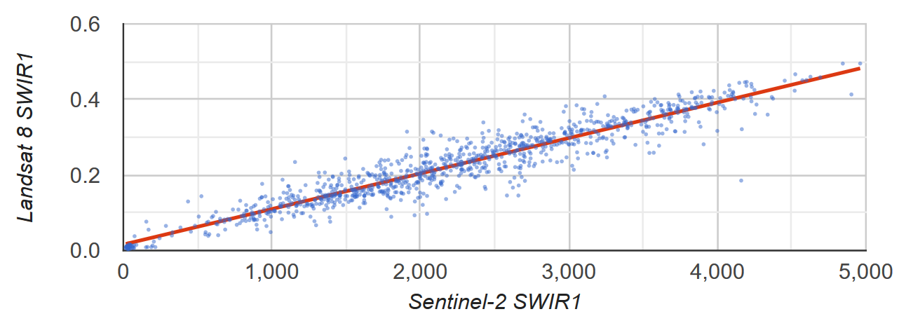
Hình 2. Biểu đồ tán xạ và đường hồi quy tuyến tính bình phương nhỏ nhất cho một mẫu pixel đại diện cho độ phản chiếu TOA của Sentinel-2 và Landsat 8 SWIR1.
ee.List
Cột của đối tượng ee.List 2D có thể là dữ liệu đầu vào cho các hàm rút gọn hồi quy. Các ví dụ sau đây cung cấp bằng chứng đơn giản; biến độc lập là một bản sao của biến phụ thuộc tạo ra một giá trị y-intercept bằng 0 và độ dốc bằng 1.
linearFit()
Trình soạn thảo mã (JavaScript)
// Define a list of lists, where columns represent variables. The first column
// is the independent variable and the second is the dependent variable.
var listsVarColumns = ee.List([
  [1, 1],
  [2, 2],
  [3, 3],
  [4, 4],
  [5, 5]
]);

// Compute the least squares estimate of a linear function. Note that an
// object is returned; cast it as an ee.Dictionary to make accessing the
// coefficients easier.
var linearFit = ee.Dictionary(listsVarColumns.reduce(ee.Reducer.linearFit()));

// Inspect the result.
print(linearFit);
print('y-intercept:', linearFit.get('offset'));
print('Slope:', linearFit.get('scale'));
Chuyển đổi danh sách nếu các biến được biểu thị bằng hàng bằng cách chuyển đổi thành ee.Array, chuyển đổi danh sách đó, sau đó chuyển đổi lại thành ee.List.
Trình soạn thảo mã (JavaScript)
// If variables in the list are arranged as rows, you'll need to transpose it.
// Define a list of lists where rows represent variables. The first row is the
// independent variable and the second is the dependent variable.
var listsVarRows = ee.List([
  [1, 2, 3, 4, 5],
  [1, 2, 3, 4, 5]
]);

// Cast the ee.List as an ee.Array, transpose it, and cast back to ee.List.
var listsVarColumns = ee.Array(listsVarRows).transpose().toList();

// Compute the least squares estimate of a linear function. Note that an
// object is returned; cast it as an ee.Dictionary to make accessing the
// coefficients easier.
var linearFit = ee.Dictionary(listsVarColumns.reduce(ee.Reducer.linearFit()));

// Inspect the result.
print(linearFit);
print('y-intercept:', linearFit.get('offset'));
print('Slope:', linearFit.get('scale'));
linearRegression()
Việc áp dụng ee.Reducer.linearRegression() tương tự như ví dụ linearFit() ở trên, ngoại trừ việc có một biến độc lập không đổi.
Trình soạn thảo mã (JavaScript)
// Define a list of lists where columns represent variables. The first column
// represents a constant term, the second an independent variable, and the third
// a dependent variable.
var listsVarColumns = ee.List([
  [1, 1, 1],
  [1, 2, 2],
  [1, 3, 3],
  [1, 4, 4],
  [1, 5, 5]
]);

// Compute ordinary least squares regression coefficients. numX is 2 because
// there is one constant term and an additional independent variable. numY is 1
// because there is only a single dependent variable. Cast the resulting
// object to an ee.Dictionary for easy access to the properties.
var linearRegression = ee.Dictionary(
  listsVarColumns.reduce(ee.Reducer.linearRegression({
    numX: 2,
    numY: 1
})));

// Convert the coefficients array to a list.
var coefList = ee.Array(linearRegression.get('coefficients')).toList();

// Extract the y-intercept and slope.
var b0 = ee.List(coefList.get(0)).get(0); // y-intercept
var b1 = ee.List(coefList.get(1)).get(0); // slope

// Extract the residuals.
var residuals = ee.Array(linearRegression.get('residuals')).toList().get(0);

// Inspect the results.
print('OLS estimates', linearRegression);
print('y-intercept:', b0);
print('Slope:', b1);
print('Residuals:', residuals);