이전에는 다음과 같이 하여 개별 Landsat 장면을 가져오는 방법을 배웠습니다.
여기서 l8 및 point는 Landsat 8 TOA 컬렉션과 관심 영역 지오메트리를 나타내는 가져오기입니다.
코드 편집기 (JavaScript)
// Define a point of interest. Use the UI Drawing Tools to import a point// geometry and name it "point" or set the point coordinates with the// ee.Geometry.Point() function as demonstrated here.varpoint=ee.Geometry.Point([-122.292,37.9018]);// Import the Landsat 8 TOA image collection.varl8=ee.ImageCollection('LANDSAT/LC08/C02/T1_TOA');// Get the least cloudy image in 2015.varimage=ee.Image(l8.filterBounds(point).filterDate('2015-01-01','2015-12-31').sort('CLOUD_COVER').first());
이제 Landsat 이미지에서 정규 식생 지수 (NDVI) 이미지를 계산한다고 가정해 보겠습니다. 식물은 전자기 스펙트럼의 근적외선 (NIR) 부분에서 빛을 반사하고 빨간색 부분에서 빛을 흡수합니다 (식물의 NIR 반사율 자세히 알아보기). NDVI는 이를 사용하여 픽셀에서 발생하는 광합성 활동을 대략적으로 반영하는 단일 값을 생성합니다. 계산은 (NIR - red) / (NIR + red)입니다. 이로 인해 1과 -1 사이의 값이 생성되며, 광합성 활동이 높은 픽셀은 NDVI가 높습니다. 다음은 Earth Engine에서 NDVI를 계산하는 한 가지 방법입니다.
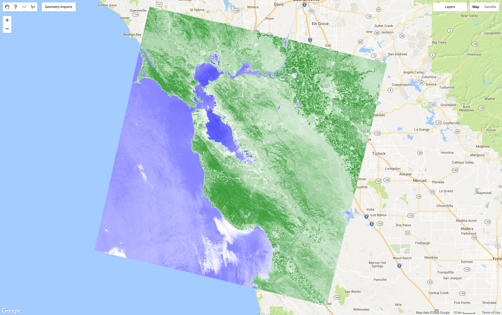
결과는 그림 8과 같이 표시됩니다. 마스크에 관한 이전 섹션에서 알아본 select() 함수를 사용하여 NIR 및 빨간색 밴드를 가져온 다음 Image 수학에 관한 섹션에서 이전에 본 이미지 수학 연산자를 사용하여 NDVI를 계산합니다. 마지막으로 팔레트를 사용하여 이미지를 표시합니다. 여기서는 팔레트에서 16진수 문자열 대신 색상 이름을 사용했습니다. (자세한 내용은 CSS 색상에 관한 외부 참조를 참고하세요.)
그림 8. 단일 Landsat 장면의 NDVI입니다. 파란색은 NDVI가 낮고 녹색은 NDVI가 높습니다.
정규화된 차이 연산은 원격 감지에서 매우 일반적이므로 이전 예의 코드를 간소화하는 데 유용한 ee.Image의 단축키 함수가 있습니다.
이제 이미지 컬렉션의 모든 이미지에 NDVI를 추가한다고 가정해 보겠습니다. Earth Engine에서 이 작업을 수행하는 방법은 컬렉션에서 함수를 map()하는 것입니다.
map()를 Map 객체와 혼동하지 마세요. 전자는 컬렉션의 메서드이며 컬렉션의 모든 요소에 함수를 적용하는 병렬 컴퓨팅 의미에서 map을 사용합니다. 이 함수는 컬렉션의 모든 요소에 적용될 작업을 정의합니다. JavaScript 튜토리얼의 간단한 함수를 살펴봤지만 이제 Earth Engine 기능을 포함하는 함수를 만들어 보겠습니다. 예를 들어 이전 NDVI 코드를 NDVI 밴드가 있는 입력 이미지를 반환하는 함수에 복사합니다.
이 코드는 단일 이미지의 NDVI를 계산하는 데는 효율적이지 않을 수 있지만 이 함수를 map()의 인수로 사용하여 컬렉션의 모든 이미지에 NDVI 밴드를 추가할 수 있습니다. 함수가 예상대로 작동하는지 확인하기 위해 단일 이미지에서 먼저 함수를 테스트하는 것이 유용할 때가 많습니다. 개별 이미지에서 함수를 테스트하고 원하는 대로 작동하는지 확인한 후에는 컬렉션에 매핑할 수 있습니다.
이 컬렉션의 모든 이미지에 NDVI 밴드가 실제로 배치되는지 확인하려면 withNDVI 컬렉션을 지도에 추가하고 인스펙터 탭으로 임의의 위치를 쿼리하면 됩니다. 이제 컬렉션의 각 이미지에 NDVI라는 밴드가 있습니다.
가장 푸른 픽셀 합성 만들기
이제 각 이미지에 NDVI 밴드가 있는 이미지 컬렉션을 만들었으므로 qualityMosaic()를 사용하여 컴포지션을 만드는 새로운 방법을 살펴볼 수 있습니다. 중간 픽셀 컴포지트에서도 Landsat 경로 간 불연속성이 나타날 수 있습니다. 이는 인접한 경로의 이미지가 서로 다른 시간 (특히 8일 차이)에 수집되어 생태학에 차이가 있기 때문일 수 있습니다. 이를 최소화하는 한 가지 방법은 식물의 최대 녹색도 시기 (잎이 있고 광합성 활동이 활발한 시기)와 같이 대략 동일한 생물 계절학적 단계에서 합성의 픽셀 값을 설정하는 것입니다. 최대 녹색도를 최대 NDVI로 정의하면 qualityMosaic()를 사용하여 각 픽셀에 컬렉션의 최대 NDVI 픽셀이 포함된 컴포지션을 만들 수 있습니다.
이제 withNDVI 컬렉션에서 추가된 NDVI 밴드를 사용할 수 있습니다.
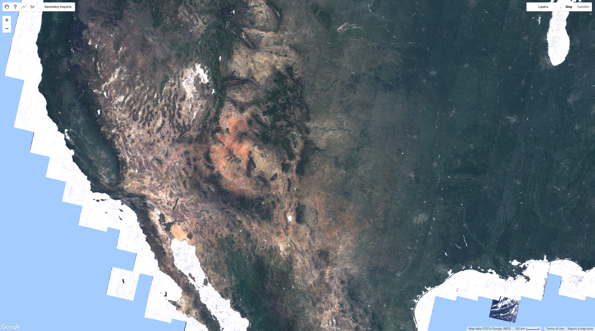
이 코드의 결과는 그림 9와 같습니다. 그림 9를 그림 6에 표시된 중간 복합 이미지와 비교하면 가장 녹색인 픽셀 복합 이미지가 실제로 훨씬 더 녹색임을 알 수 있습니다. 하지만 수역을 자세히 살펴보면 다른 문제가 드러날 수 있습니다. 특히 수역이 흐리게 표시됩니다. 이는 qualityMosaic() 메서드의 작동 방식 때문입니다. 각 위치에서 전체 시계열이 검사되고 NDVI 밴드에서 최댓값을 갖는 픽셀이 합성 값으로 설정됩니다. NDVI는 물보다 구름에서 더 높기 때문에 물 영역은 흐린 픽셀을 갖게 되며, 식물이 있는 영역은 모두 녹색으로 표시됩니다. 픽셀의 식물이 광합성으로 활성화되어 있을 때 NDVI가 가장 높기 때문입니다.
그림 9. Landsat 8 가장 푸른 픽셀 합성
이제 Earth Engine에서 이미지를 합성하고 모자이크하는 여러 방법을 살펴보았습니다. 시간과 장소로 필터링된 이미지 또는 컬렉션의 모든 이미지에서 최근 값, 중앙값 또는 가장 녹색인 픽셀 합성 이미지를 만들 수 있습니다. 이미지에서 계산을 수행하고 정보를 추출하는 방법을 배웠습니다. 다음 페이지에서는 Earth Engine에서 정보를 가져오는 방법(예: Google Drive 폴더로 내보낸 차트 또는 데이터 세트)을 다룹니다.
[null,null,["최종 업데이트: 2025-07-26(UTC)"],[[["\u003cp\u003eThis guide explains how to calculate and add an NDVI (Normalized Difference Vegetation Index) band to Landsat 8 imagery in Earth Engine.\u003c/p\u003e\n"],["\u003cp\u003eIt demonstrates how to use the \u003ccode\u003emap()\u003c/code\u003e function to apply a custom function, like NDVI calculation, to every image in a collection.\u003c/p\u003e\n"],["\u003cp\u003eThe tutorial explores creating a "greenest-pixel" composite using \u003ccode\u003equalityMosaic()\u003c/code\u003e to highlight areas with peak vegetation.\u003c/p\u003e\n"],["\u003cp\u003eIt highlights the potential issues with using \u003ccode\u003equalityMosaic()\u003c/code\u003e for compositing, such as cloud contamination in water bodies due to NDVI values.\u003c/p\u003e\n"],["\u003cp\u003eUsers are encouraged to further explore data extraction and visualization techniques in subsequent tutorials.\u003c/p\u003e\n"]]],[],null,["# NDVI, Mapping a Function over a Collection, Quality Mosaicking\n\nPreviously, you learned how to get individual Landsat scenes by doing something like this,\nwhere `l8` and `point` are imports representing the Landsat 8 TOA\ncollection and an area-of-interest geometry:\n\n\n### Code Editor (JavaScript)\n\n```javascript\n// Define a point of interest. Use the UI Drawing Tools to import a point\n// geometry and name it \"point\" or set the point coordinates with the\n// ee.Geometry.Point() function as demonstrated here.\nvar point = ee.Geometry.Point([-122.292, 37.9018]);\n\n// Import the Landsat 8 TOA image collection.\nvar l8 = ee.ImageCollection('LANDSAT/LC08/C02/T1_TOA');\n\n// Get the least cloudy image in 2015.\nvar image = ee.Image(\n l8.filterBounds(point)\n .filterDate('2015-01-01', '2015-12-31')\n .sort('CLOUD_COVER')\n .first()\n);\n```\n\nSuppose now that you want to compute a Normalized Difference Vegetation Index (NDVI)\nimage from the Landsat image. Vegetation reflects light in the\nnear-infrared (NIR) part of the electromagnetic spectrum and absorbs light in the red\npart ([Learn more about NIR\nreflectance from vegetation](https://science.nasa.gov/ems/08_nearinfraredwaves)). NDVI uses this to create a single value roughly\nreflecting the photosynthetic activity occurring at a pixel. The calculation is\n(NIR - red) / (NIR + red). This results in a number between 1 and -1, where pixels with\nhigh photosynthetic activity have a high NDVI. This is one way to compute NDVI in Earth\nEngine:\n\n### Code Editor (JavaScript)\n\n```javascript\n// Compute the Normalized Difference Vegetation Index (NDVI).\nvar nir = image.select('B5');\nvar red = image.select('B4');\nvar ndvi = nir.subtract(red).divide(nir.add(red)).rename('NDVI');\n\n// Display the result.\nMap.centerObject(image, 9);\nvar ndviParams = {min: -1, max: 1, palette: ['blue', 'white', 'green']};\nMap.addLayer(ndvi, ndviParams, 'NDVI image');\n```\n\nThe result should look something like Figure 8. Note that we use the `select()`\nfunction you learned about in the [previous section on\nmasking](/earth-engine/tutorials/tutorial_api_05#masking) to get the NIR and red bands, then compute NDVI using image mathematical\noperators that that you have also [seen before in\nthe section on `Image` math](/earth-engine/tutorials/tutorial_api_03#image-math). Finally, display the image with a palette. Here\nwe used color names instead of hex strings in the palette. (See\n[this external\nreference about CSS color](https://developer.mozilla.org/en-US/docs/Web/CSS/color_value) for details.)\nFigure 8. NDVI for a single Landsat scene. Blue is low and green is high NDVI.\n\nThe normalized difference operation is so ubiquitous in remote sensing, there is a\n[shortcut function](/earth-engine/apidocs/ee-image-normalizeddifference) on an\n`ee.Image` that is useful for simplifying the code in the previous example:\n\n### Code Editor (JavaScript)\n\n```javascript\nvar ndvi = image.normalizedDifference(['B5', 'B4']).rename('NDVI');\n```\n\nMapping a Function over a Collection\n------------------------------------\n\nSuppose now that you want to add NDVI to *every* image in an image collection. The\nway to do that in Earth Engine is to `map()` a function over the collection.\nDon't confuse `map()` with the `Map` object. The former is a method\non a collection, and uses *map* in the\n[parallel computing sense](https://en.wikipedia.org/wiki/Map_(parallel_pattern))\nof applying a function to every element in a collection. The function defines the\noperations that will be applied to every element in the collection. You have seen\n[a simple function in the JavaScript tutorial](/earth-engine/tutorials/tutorial_js_01#functions), but\nnow we're going to make a function that includes Earth Engine functionality. For example,\ncopy the previous NDVI code into a function which returns the input image with an NDVI band:\n\n### Code Editor (JavaScript)\n\n```javascript\nvar addNDVI = function(image) {\n var ndvi = image.normalizedDifference(['B5', 'B4']).rename('NDVI');\n return image.addBands(ndvi);\n};\n\n// Test the addNDVI function on a single image.\nvar ndvi = addNDVI(image).select('NDVI');\n```\n\nThis code might not be as efficient for computing NDVI for a single image, but this\nfunction can be used as an argument to `map()` in order to add an NDVI band\nto every image in the collection. It's often useful to first test a function on a single\nimage, to make sure the function is behaving as you expect. Once you've tested the function\non an individual image and have determined that it does what you want, you can map it\nover the collection:\n\n### Code Editor (JavaScript)\n\n```javascript\nvar withNDVI = l8.map(addNDVI);\n```\n\nTo verify that this is indeed putting an NDVI band in every image in this collection,\nyou can add the `withNDVI` collection to the map and query a random location\nwith the **Inspector** tab. You should notice that each image in the\ncollection now has a band called `NDVI`.\n\nMake a greenest pixel composite\n-------------------------------\n\nNow that you've made an image collection in which each image has an NDVI band, we can\nexplore a new way to make composites: `qualityMosaic()`. You may have noticed\ndiscontinuities between Landsat paths, even in the median pixel composite. Part of the\nreason for that may be due to differences in\n[phenology](https://en.wikipedia.org/wiki/Phenology) as a result of images in\nadjacent paths being collected at different times (specifically, 8 days apart). One way to\nminimize this is to try to set pixel values in the composite from roughly the same\nphenological stage, for example the time of maximum greenness of plants (when the leaves\nare on and photosynthetically active). If we let max greenness be defined by the maximum\nNDVI, we can use\n[`qualityMosaic()`](/earth-engine/apidocs/ee-imagecollection-qualitymosaic) to\nmake a composite in which each pixel contains the maximum NDVI pixel from the collection.\nNow you can make use of the added NDVI band in your `withNDVI` collection:\n\n### Code Editor (JavaScript)\n\n```javascript\n// Make a \"greenest\" pixel composite.\nvar greenest = withNDVI.qualityMosaic('NDVI');\n\n// Display the result.\nvar visParams = {bands: ['B4', 'B3', 'B2'], max: 0.3};\nMap.addLayer(greenest, visParams, 'Greenest pixel composite');\n```\n\nThe result of this code should look something like Figure 9. Comparing Figure 9 to the\nmedian composite shown in [Figure 6](/earth-engine/tutorials/tutorial_api_05#compositing-with-reducers),\nobserve that the greenest pixel composite is indeed much greener. However, close\nexamination of water bodies should make a different problem apparent. Specifically,\nwater bodies now appear cloudy. This is due to the way the `qualityMosaic()`\nmethod works: at each location, the entire time series is examined and the pixel with the\nmaximum value in the NDVI band is set as the composite value. Because NDVI is higher over\nclouds than water, water areas get cloudy pixels, while vegetated areas all appear green\nbecause NDVI is highest when the vegetation in the pixel is photosynthetically active.\nFigure 9. Landsat 8 greenest pixel composite.\n\nNow you've seen several ways to composite and mosaic images in Earth Engine. You can make\nrecent-value, median, or greenest-pixel composites from images filtered by time and place\nor all images in the collection. You've learned how to do computations on the imagery and\nextract information. The next page covers ways to get information out of Earth Engine, for\nexample as a chart or a dataset exported to your Google Drive folder. \n[arrow_backPrevious page](/earth-engine/tutorials/tutorial_api_05) [Next pagearrow_forward](/earth-engine/tutorials/tutorial_api_07)"]]