Intensidad del cambio en la ocurrencia de agua

La capa de datos de Intensidad del cambio en la ocurrencia de agua proporciona una medida de cómo cambió el agua superficial entre dos épocas: 1984-1999 y 2000-2015. La capa calcula el promedio del cambio en pares homólogos de meses tomados de las dos épocas. Consulta la Guía de usuarios de datos (v2) para obtener más detalles sobre esta capa.

En esta sección del instructivo, se hará lo siguiente:

1. Agregar una capa de mapa con diseño para visualizar la intensidad del cambio en la presencia de agua
2. Resumir la intensidad del cambio en una región de interés especificada con un histograma

Visualización

Al igual que con la capa de ocurrencia de agua, comenzaremos por agregar una visualización básica de la intensidad del cambio de ocurrencia al mapa y, luego, la mejoraremos. La intensidad del cambio de ocurrencia se proporciona de dos maneras, tanto como valores absolutos como normalizados. En este instructivo, usaremos los valores absolutos. Para comenzar, selecciona la capa de intensidad del cambio de ocurrencia absoluto en la imagen de GSW:

Editor de código (JavaScript)

var change = gsw.select("change_abs");

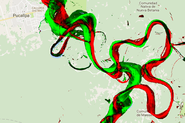
En la sección Constants del código, agrega una instrucción que cree una variable nueva que defina cómo se aplicará el diseño de la capa. Este diseño muestra las áreas en las que la presencia de agua superficial disminuyó o aumentó en rojo o verde, respectivamente. Las áreas en las que la presencia de agua superficial no cambió significativamente se muestran en negro.

Editor de código (JavaScript)

var VIS_CHANGE = {
    min:-50,
    max:50,
    palette: ['red', 'black', 'limegreen']
};

Al final de la sección Map Layers del código, agrega una instrucción que agregue una nueva capa al mapa.

Editor de código (JavaScript)

Map.setCenter(-74.4557, -8.4289, 11);  // Ucayali River, Peru
Map.addLayer({
  eeObject: change,
  visParams: VIS_CHANGE,
  name: 'occurrence change intensity'
});

Figura 6. Captura de pantalla de la intensidad del cambio del agua superficial del río Ucayali cerca de Pucallpa, una ciudad en la selva amazónica del este de Perú. El rojo y el verde indican una disminución o un aumento en la presencia de agua superficial entre las épocas.

Resumen del cambio dentro de una región de interés

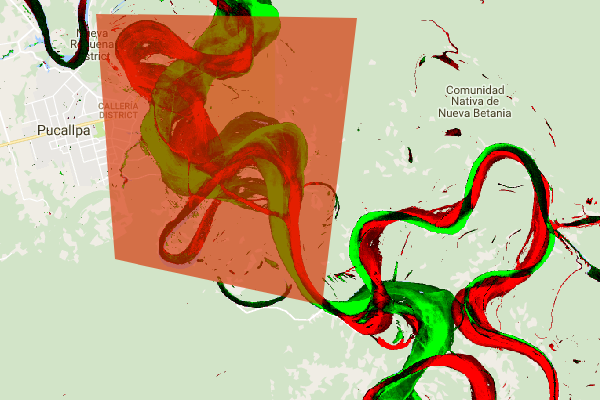
En esta sección, resumiremos la cantidad de cambio dentro de una región de interés especificada. Para especificar una región de interés, haz clic en la herramienta de dibujo de polígonos, que es una de las Herramientas de geometría. Esto creará una nueva capa Geometry Imports, que se llamará "geometry" de forma predeterminada. Para cambiar el nombre, haz clic en el ícono de ajustes ubicado a la derecha del nombre de la capa. (Ten en cuenta que es posible que debas colocar el cursor sobre el nombre de la capa para que aparezca).

Cambia el nombre de la capa a roi (para la región de interés o ROI). Luego, podemos hacer clic en una serie de puntos en el mapa para definir una región de interés poligonal.

Figura 7. Captura de pantalla del río Ucayali cerca de Pucallpa, Perú, con una región de interés creada con la herramienta de dibujo de polígonos.

Ahora que nuestra región de interés está definida y almacenada en una variable, podemos usarla para calcular un histograma de la intensidad del cambio para la ROI. Agrega el siguiente código a la sección Calculations de la secuencia de comandos.

Editor de código (JavaScript)

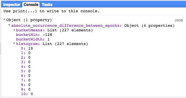
// Calculate a change intensity for the region of interest.
var histogram = change.reduceRegion({
  reducer: ee.Reducer.histogram(),
  geometry: roi,
  scale: 30,
  bestEffort: true,
});
print(histogram);

La primera instrucción calcula un histograma de los valores de intensidad del cambio de ocurrencia dentro del ROI, con un muestreo a una escala de 30 m. El segundo imprime el objeto resultante en la pestaña de la consola del editor de código. Puedes expandir el árbol de objetos para ver los valores de los buckets del histograma. Los datos numéricos están ahí, pero hay mejores maneras de visualizar los resultados.

Figura 8. Resultados de la pestaña de la consola, que muestran los valores del histograma de la intensidad del cambio en el agua superficial.

Para mejorar esto, podemos generar un gráfico de histograma. Reemplaza la instrucción que define el objeto de histograma por las siguientes instrucciones:

Editor de código (JavaScript)

// Generate a histogram object and print it to the console tab.
var histogram = ui.Chart.image.histogram({
  image: change,
  region: roi,
  scale: 30,
  minBucketWidth: 10
});
histogram.setOptions({
  title: 'Histogram of surface water change intensity.'
});

Estas instrucciones crean un objeto de gráfico de histograma, que reemplaza el árbol de objetos de histograma en la pestaña Console por un gráfico. El método del gráfico contiene varios argumentos, incluidos scale, que define la escala espacial, en metros, en la que se muestrea la región de interés, y minBucketWidth, que se usa para controlar el ancho de los buckets del histograma.

Figura 9. Resultados de la pestaña de la consola, que muestran un gráfico de histograma de la intensidad del cambio del agua superficial.

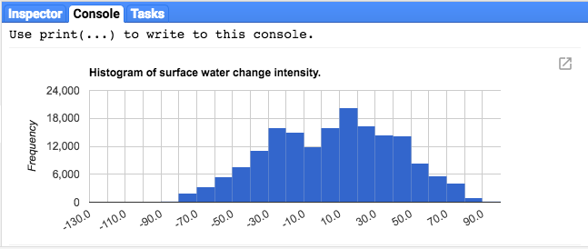
Puedes explorar los valores del gráfico de forma interactiva colocando el cursor sobre las barras del histograma.

Guion final

A continuación, se incluye el guion completo de esta sección. Ten en cuenta que la secuencia de comandos incluye instrucciones para definir una geometría de polígono (roi), que es comparable a la geometría que creaste con las herramientas de geometría del editor de código.

Editor de código (JavaScript)

//////////////////////////////////////////////////////////////
// Asset List
//////////////////////////////////////////////////////////////

var gsw = ee.Image('JRC/GSW1_0/GlobalSurfaceWater');
var occurrence = gsw.select('occurrence');
var change = gsw.select("change_abs");
var roi = /* color: 0B4A8B */ee.Geometry.Polygon(
        [[[-74.17213, -8.65569],
          [-74.17419, -8.39222],
          [-74.38362, -8.36980],
          [-74.43031, -8.61293]]]);

//////////////////////////////////////////////////////////////
// Constants
//////////////////////////////////////////////////////////////

var VIS_OCCURRENCE = {
    min:0,
    max:100,
    palette: ['red', 'blue']
};
var VIS_CHANGE = {
    min:-50,
    max:50,
    palette: ['red', 'black', 'limegreen']
};
var VIS_WATER_MASK = {
  palette: ['white', 'black']
};

//////////////////////////////////////////////////////////////
// Calculations
//////////////////////////////////////////////////////////////

// Create a water mask layer, and set the image mask so that non-water areas are transparent.
var water_mask = occurrence.gt(90).mask(1);

// Generate a histogram object and print it to the console tab.
var histogram = ui.Chart.image.histogram({
  image: change,
  region: roi,
  scale: 30,
  minBucketWidth: 10
});
histogram.setOptions({
  title: 'Histogram of surface water change intensity.'
});
print(histogram);

//////////////////////////////////////////////////////////////
// Initialize Map Location
//////////////////////////////////////////////////////////////

// Uncomment one of the following statements to center the map on
// a particular location.
// Map.setCenter(-90.162, 29.8597, 10);   // New Orleans, USA
// Map.setCenter(-114.9774, 31.9254, 10); // Mouth of the Colorado River, Mexico
// Map.setCenter(-111.1871, 37.0963, 11); // Lake Powell, USA
// Map.setCenter(149.412, -35.0789, 11);  // Lake George, Australia
// Map.setCenter(105.26, 11.2134, 9);     // Mekong River Basin, SouthEast Asia
// Map.setCenter(90.6743, 22.7382, 10);   // Meghna River, Bangladesh
// Map.setCenter(81.2714, 16.5079, 11);   // Godavari River Basin Irrigation Project, India
// Map.setCenter(14.7035, 52.0985, 12);   // River Oder, Germany & Poland
// Map.setCenter(-59.1696, -33.8111, 9);  // Buenos Aires, Argentina\
Map.setCenter(-74.4557, -8.4289, 11);  // Ucayali River, Peru

//////////////////////////////////////////////////////////////
// Map Layers
//////////////////////////////////////////////////////////////

Map.addLayer({
  eeObject: water_mask,
  visParams: VIS_WATER_MASK,
  name: '90% occurrence water mask',
  shown: false
});
Map.addLayer({
  eeObject: occurrence.updateMask(occurrence.divide(100)),
  name: "Water Occurrence (1984-2015)",
  visParams: VIS_OCCURRENCE,
  shown: false
});
Map.addLayer({
  eeObject: change,
  visParams: VIS_CHANGE,
  name: 'occurrence change intensity'
});

En la siguiente sección, explorarás más a fondo cómo cambió el agua con el tiempo trabajando con la capa de transición de la clase de agua.