 GitHub でソースを見る
画像オブジェクトは、同じ整数値を持つ接続されたピクセルのセットです。カテゴリ、ビン、ブール値の画像データは、オブジェクト分析に適しています。
Earth Engine には、各オブジェクトに固有の ID をラベル付けするメソッド、オブジェクトを構成するピクセル数をカウントするメソッド、オブジェクトと交差するピクセルの値の統計情報を計算するメソッドが用意されています。
connectedComponents(): 各オブジェクトに一意の ID をラベル付けします。connectedPixelCount(): 各オブジェクトのピクセル数を計算します。reduceConnectedComponents(): 各オブジェクト内のピクセルの統計情報を計算します。
熱のホットスポット
以降のセクションでは、Landsat 8 の表面温度に適用されるオブジェクトベースの方法の例を示します。各セクションは前のセクションを基にしています。次のスニペットを実行して、サンフランシスコの小さな地域の熱ホットスポット(303 ケルビン超)のベース画像を生成します。
コードエディタ(JavaScript)
// Make an area of interest geometry centered on San Francisco.
var point = ee.Geometry.Point(-122.1899, 37.5010);
var aoi = point.buffer(10000);

// Import a Landsat 8 image, subset the thermal band, and clip to the
// area of interest.
var kelvin = ee.Image('LANDSAT/LC08/C02/T1_TOA/LC08_044034_20140318')
  .select(['B10'], ['kelvin'])
  .clip(aoi);

// Display the thermal band.
Map.centerObject(point, 13);
Map.addLayer(kelvin, {min: 288, max: 305}, 'Kelvin');

// Threshold the thermal band to set hot pixels as value 1, mask all else.
var hotspots = kelvin.gt(303)
  .selfMask()
  .rename('hotspots');

// Display the thermal hotspots on the Map.
Map.addLayer(hotspots, {palette: 'FF0000'}, 'Hotspots');
import ee
import geemap.core as geemap
Colab(Python)
# Make an area of interest geometry centered on San Francisco.
point = ee.Geometry.Point(-122.1899, 37.5010)
aoi = point.buffer(10000)

# Import a Landsat 8 image, subset the thermal band, and clip to the
# area of interest.
kelvin = (
    ee.Image('LANDSAT/LC08/C02/T1_TOA/LC08_044034_20140318')
    .select(['B10'], ['kelvin'])
    .clip(aoi)
)

# Threshold the thermal band to set hot pixels as value 1, mask all else.
hotspots = kelvin.gt(303).selfMask().rename('hotspots')

# Define a map centered on Redwood City, California.
map_objects = geemap.Map(center=[37.5010, -122.1899], zoom=13)

# Add the image layers to the map.
map_objects.add_layer(kelvin, {'min': 288, 'max': 305}, 'Kelvin')
map_objects.add_layer(hotspots, {'palette': 'FF0000'}, 'Hotspots')

図 1. サンフランシスコの地域の気温。温度が 303 ケルビンを超えるピクセルは赤色で示されます(熱的なホットスポット)。
オブジェクトにラベルを付ける
多くの場合、オブジェクトの分析の最初のステップはオブジェクトのラベル付けです。ここでは、connectedComponents() 関数を使用して画像オブジェクトを識別し、それぞれに一意の ID を割り当てます。オブジェクトに属するすべてのピクセルに同じ整数 ID 値が割り当てられます。結果は、画像の最初のバンドのピクセルの接続に基づいてピクセルをオブジェクト ID 値に関連付ける「ラベル」バンドが追加された入力画像のコピーです。
コードエディタ(JavaScript)
// Uniquely label the hotspot image objects.
var objectId = hotspots.connectedComponents({
  connectedness: ee.Kernel.plus(1),
  maxSize: 128
});

// Display the uniquely ID'ed objects to the Map.
Map.addLayer(objectId.randomVisualizer(), null, 'Objects');
import ee
import geemap.core as geemap
Colab(Python)
# Uniquely label the hotspot image objects.
object_id = hotspots.connectedComponents(
    connectedness=ee.Kernel.plus(1), maxSize=128
)

# Add the uniquely ID'ed objects to the map.
map_objects.add_layer(object_id.randomVisualizer(), None, 'Objects')
パッチの最大サイズは 128 ピクセルに設定されています。それより多くのピクセルで構成されるオブジェクトはマスクされます。接続は ee.Kernel.plus(1) カーネルで指定します。これは 4 隣接接続を定義します。8 隣接の場合は ee.Kernel.square(1) を使用します。

図 2. 一意の ID でラベル付けされ、スタイル設定されたサーマル ホットスポット オブジェクト。
オブジェクト サイズ
ピクセル数
connectedPixelCount() イメージ メソッドを使用して、オブジェクトを構成するピクセル数を計算します。オブジェクト内のピクセル数を知ることは、サイズでオブジェクトをマスクしたり、オブジェクト領域を計算したりする際に役立ちます。次のスニペットは、前のセクションで定義した objectId イメージの「ラベル」バンドに connectedPixelCount() を適用します。
コードエディタ(JavaScript)
// Compute the number of pixels in each object defined by the "labels" band.
var objectSize = objectId.select('labels')
  .connectedPixelCount({
    maxSize: 128, eightConnected: false
  });

// Display object pixel count to the Map.
Map.addLayer(objectSize, null, 'Object n pixels');
import ee
import geemap.core as geemap
Colab(Python)
# Compute the number of pixels in each object defined by the "labels" band.
object_size = object_id.select('labels').connectedPixelCount(
    maxSize=128, eightConnected=False
)

# Add the object pixel count to the map.
map_objects.add_layer(object_size, None, 'Object n pixels')
connectedPixelCount() は、各バンドの各ピクセルに、eightConnected パラメータに渡されたブール値引数によって決定される 4 つまたは 8 つの隣接接続ルールに従って接続された隣接ピクセルの数を含む入力画像のコピーを返します。接続は、入力画像のバンドごとに個別に決定されます。この例では、オブジェクト ID を表す単一バンド画像(objectId)が入力として提供されたため、単一バンド画像が「ラベル」バンド(入力画像に存在)とともに返されましたが、値はオブジェクトを構成するピクセル数を表します。各オブジェクトのすべてのピクセルは同じピクセル数値を持ちます。

図 3. サイズ別にラベルが付けられ、スタイル設定されたサーマル ホットスポット オブジェクト。
地域
オブジェクト領域は、1 つのピクセルの面積に、オブジェクトを構成するピクセル数(connectedPixelCount() によって決定)を掛けて計算します。ピクセル領域は、ee.Image.pixelArea() から生成された画像によって提供されます。
コードエディタ(JavaScript)
// Get a pixel area image.
var pixelArea = ee.Image.pixelArea();

// Multiply pixel area by the number of pixels in an object to calculate
// the object area. The result is an image where each pixel
// of an object relates the area of the object in m^2.
var objectArea = objectSize.multiply(pixelArea);

// Display object area to the Map.
Map.addLayer(objectArea,
             {min: 0, max: 30000, palette: ['0000FF', 'FF00FF']},
             'Object area m^2');
import ee
import geemap.core as geemap
Colab(Python)
# Get a pixel area image.
pixel_area = ee.Image.pixelArea()

# Multiply pixel area by the number of pixels in an object to calculate
# the object area. The result is an image where each pixel
# of an object relates the area of the object in m^2.
object_area = object_size.multiply(pixel_area)

# Add the object area to the map.
map_objects.add_layer(
    object_area,
    {'min': 0, 'max': 30000, 'palette': ['0000FF', 'FF00FF']},
    'Object area m^2',
)
結果は、オブジェクトの各ピクセルがオブジェクトの面積(平方メートル)を表す画像です。この例では、objectSize 画像には単一のバンドが含まれています。マルチバンドの場合は、乗算演算が画像の各バンドに適用されます。
サイズでオブジェクトをフィルタする
オブジェクトのサイズは、特定のサイズのオブジェクトに分析を集中させるマスク条件として使用できます(サイズが小さすぎるオブジェクトをマスクアウトするなど)。ここでは、前の手順で計算した objectArea 画像がマスクとして使用され、面積が 1 ヘクタール未満のオブジェクトが削除されます。
コードエディタ(JavaScript)
// Threshold the `objectArea` image to define a mask that will mask out
// objects below a given size (1 hectare in this case).
var areaMask = objectArea.gte(10000);

// Update the mask of the `objectId` layer defined previously using the
// minimum area mask just defined.
objectId = objectId.updateMask(areaMask);
Map.addLayer(objectId, null, 'Large hotspots');
import ee
import geemap.core as geemap
Colab(Python)
# Threshold the `object_area` image to define a mask that will mask out
# objects below a given size (1 hectare in this case).
area_mask = object_area.gte(10000)

# Update the mask of the `object_id` layer defined previously using the
# minimum area mask just defined.
object_id = object_id.updateMask(area_mask)
map_objects.add_layer(object_id, None, 'Large hotspots')
結果は、1 ヘクタール未満のオブジェクトがマスクされている objectId 画像のコピーです。
 |
 |
|---|---|
| 図 4a一意の ID でラベル付けされ、スタイル設定されたサーマル ホットスポット オブジェクト。 | 図 4b最小面積(1 ヘクタール)でフィルタされたサーマル ホットスポット オブジェクト。 |
ゾーン統計情報
reduceConnectedComponents() メソッドは、一意のオブジェクトを構成するピクセルにレジューサーを適用します。次のスニペットでは、これを使用してホットスポット オブジェクトの平均温度を計算します。reduceConnectedComponents() では、圧縮するバンド(またはバンド)と、オブジェクトラベルを定義するバンドを含む入力画像が必要です。ここでは、objectID「ラベル」画像バンドが kelvin 温度画像に追加され、適切な入力画像が作成されます。
コードエディタ(JavaScript)
// Make a suitable image for `reduceConnectedComponents()` by adding a label
// band to the `kelvin` temperature image.
kelvin = kelvin.addBands(objectId.select('labels'));

// Calculate the mean temperature per object defined by the previously added
// "labels" band.
var patchTemp = kelvin.reduceConnectedComponents({
  reducer: ee.Reducer.mean(),
  labelBand: 'labels'
});

// Display object mean temperature to the Map.
Map.addLayer(
  patchTemp,
  {min: 303, max: 304, palette: ['yellow', 'red']},
  'Mean temperature'
);
import ee
import geemap.core as geemap
Colab(Python)
# Make a suitable image for `reduceConnectedComponents()` by adding a label
# band to the `kelvin` temperature image.
kelvin = kelvin.addBands(object_id.select('labels'))

# Calculate the mean temperature per object defined by the previously added
# "labels" band.
patch_temp = kelvin.reduceConnectedComponents(
    reducer=ee.Reducer.mean(), labelBand='labels'
)

# Add object mean temperature to the map and display it.
map_objects.add_layer(
    patch_temp,
    {'min': 303, 'max': 304, 'palette': ['yellow', 'red']},
    'Mean temperature',
)
display(map_objects)
結果は、オブジェクトの定義に使用されたバンドのない入力画像のコピーです。ピクセル値は、オブジェクトごと、バンドごとの減衰の結果を表します。
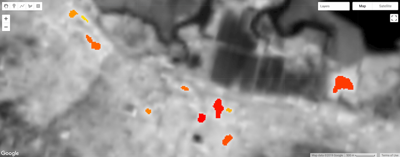
図 5. サーマル ホットスポット オブジェクトのピクセルが平均温度でまとめられ、スタイル設定されています。