شدت تغییر رخدادهای مبتنی بر آب

لایه داده‌های «شدت تغییر وقوع آب» معیاری برای نحوه تغییر آب‌های سطحی بین دو دوره زمانی ۱۹۸۴-۱۹۹۹ و ۲۰۰۰-۲۰۱۵ ارائه می‌دهد. این لایه میانگین تغییرات را در جفت ماه‌های همولوگ گرفته‌شده از دو دوره محاسبه می‌کند. برای جزئیات بیشتر درباره این لایه، راهنمای کاربران داده (نسخه ۲) را ببینید.

این بخش از آموزش:

1. یک لایه نقشه قابل‌طراحی برای تجسم شدت تغییر وقوع آب اضافه کنید، و
2. شدت تغییر را در منطقه موردنظر مشخص‌شده بااستفاده از بافت‌نگاشت خلاصه کنید.

نمایش تصویری

مشابه لایه وقوع آب، با افزودن یک تجسم اولیه از شدت تغییر وقوع به نقشه شروع می‌کنیم و سپس آن را بهبود می‌بخشیم. شدت تغییر وقوع به دو روش ارائه می‌شود، هم به‌صورت مقادیر مطلق و هم مقادیر نرمال‌شده. در این آموزش از مقادیر مطلق استفاده خواهیم کرد. با انتخاب لایه شدت تغییر وقوع مطلق از تصویر GSW شروع کنید:

ویرایشگر کد (جاوا اسکریپت)

var change = gsw.select("change_abs");

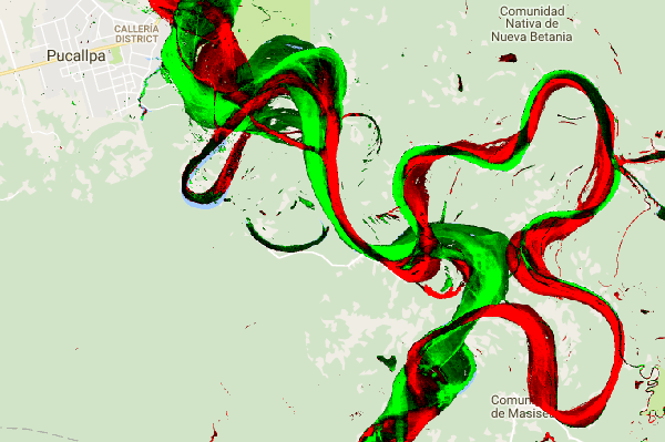
در بخش Constants (ثابت‌ها) کد، عبارتی اضافه کنید که متغیر جدیدی ایجاد کند که نحوه سبک‌بندی لایه را تعریف می‌کند. این سبک‌بندی مناطقی را نشان می‌دهد که در آن‌ها وقوع آب سطحی به رنگ قرمز/سبز کاهش/افزایش یافته است. مناطقی که وقوع آب‌های سطحی در آن‌ها نسبتاً بدون تغییر است با رنگ سیاه نشان داده شده‌اند.

ویرایشگر کد (جاوا اسکریپت)

var VIS_CHANGE = {
    min:-50,
    max:50,
    palette: ['red', 'black', 'limegreen']
};

در انتهای بخش «لایه‌های نقشه» کد، عبارتی اضافه کنید که لایه جدیدی به نقشه اضافه کند.

ویرایشگر کد (جاوا اسکریپت)

Map.setCenter(-74.4557, -8.4289, 11);  // Ucayali River, Peru
Map.addLayer({
  eeObject: change,
  visParams: VIS_CHANGE,
  name: 'occurrence change intensity'
});

شکل ۶. نماگرفتی از شدت تغییر آب سطحی برای رودخانه اوکایالی در نزدیکی پوکالپا، شهری در جنگل‌های بارانی آمازون در شرق پرو. رنگ قرمز/سبز نشان‌دهنده کاهش/افزایش وقوع آب سطحی بین دوره‌ها است.

خلاصه‌سازی تغییر در منطقه موردنظر

در این بخش، میزان تغییر را در منطقه موردنظر مشخص‌شده خلاصه می‌کنیم. برای مشخص کردن منطقه موردنظر، روی ابزار طراحی چندضلعی که یکی از ابزارهای هندسه است کلیک کنید. با این کار، لایه جدید «واردات هندسه» ایجاد می‌شود که به‌طور پیش‌فرض «هندسه» نام دارد. برای تغییر نام، روی نماد چرخ‌دنده واقع در سمت چپ نام لایه کلیک کنید. (توجه داشته باشید که ممکن است لازم باشد مکان‌نما را روی نام لایه قرار دهید تا ظاهر شود.)

نام لایه را به roi (برای منطقه موردنظر یا ROI) تغییر دهید. سپس می‌توانیم روی مجموعه‌ای از نقاط روی نقشه کلیک کنیم تا منطقه چندضلعی موردنظر را تعریف کنیم.

شکل ۷. نماگرفت از رودخانه اوکایالی در نزدیکی پوکالپا، پرو، با منطقه موردنظر ایجادشده بااستفاده از ابزار طراحی چندضلعی.

اکنون که منطقه موردنظر ما تعریف شده و در متغیری ذخیره شده است، می‌توانیم از آن برای محاسبه هیستوگرام شدت تغییر برای منطقه موردنظر استفاده کنیم. کد زیر را به بخش «محاسبات» در اسکریپت اضافه کنید.

ویرایشگر کد (جاوا اسکریپت)

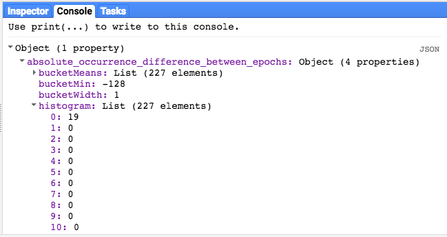
// Calculate a change intensity for the region of interest.
var histogram = change.reduceRegion({
  reducer: ee.Reducer.histogram(),
  geometry: roi,
  scale: 30,
  bestEffort: true,
});
print(histogram);

اولین عبارت، هیستوگرام مقادیر شدت تغییر وقوع را در ROI محاسبه می‌کند و در مقیاس ۳۰ متری نمونه‌برداری می‌کند. دومی شیء حاصل را در «برگه کنسول» «ویرایشگر کد» چاپ می‌کند. می‌توانید درخت شیء را ازهم باز کنید تا مقادیر سطل‌های هیستوگرام را مشاهده کنید. داده‌های عددی وجود دارد، اما روش‌های بهتری برای تجسم نتایج وجود دارد.

شکل ۸. نتایج برگه «کنسول» که مقادیر بافت‌نگاشت شدت تغییر آب‌های سطحی را نشان می‌دهد.

برای بهبود این مورد، می‌توانیم به‌جای آن نمودار هیستوگرام تولید کنیم. عبارتی را که شیء بافت‌نگاشت را تعریف می‌کند با عبارت‌های زیر جایگزین کنید:

ویرایشگر کد (جاوا اسکریپت)

// Generate a histogram object and print it to the console tab.
var histogram = ui.Chart.image.histogram({
  image: change,
  region: roi,
  scale: 30,
  minBucketWidth: 10
});
histogram.setOptions({
  title: 'Histogram of surface water change intensity.'
});

این عبارت‌ها یک شیء نمودار بافت‌نگاشت ایجاد می‌کنند که درخت شیء بافت‌نگاشت را در «زبانه کنسول» با نمودار جایگزین می‌کند. روش نمودار شامل چندین آرگومان است، ازجمله scale که مقیاس فضایی را برحسب متر تعریف می‌کند که در آن منطقه موردنظر نمونه‌برداری می‌شود، و minBucketWidth که برای کنترل عرض سطل‌های هیستوگرام استفاده می‌شود.

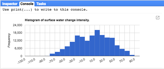
شکل ۹. نتایج برگه «کنسول» که نمودار هیستوگرام شدت تغییر آب‌های سطحی را نشان می‌دهد.

با قرار دادن مکان‌نما روی میله‌های هیستوگرام، می‌توانید مقادیر نمودار را به‌صورت تعاملی کاوش کنید.

متن نهایی

کل اسکریپت این بخش در زیر فهرست شده است. توجه داشته باشید که این اسکریپت شامل عبارت‌هایی برای تعریف هندسه چندضلعی (roi) است که با هندسه‌ای که بااستفاده از ابزارهای هندسه Code Editor ایجاد کرده‌اید قابل‌مقایسه است.

ویرایشگر کد (جاوا اسکریپت)

//////////////////////////////////////////////////////////////
// Asset List
//////////////////////////////////////////////////////////////

var gsw = ee.Image('JRC/GSW1_0/GlobalSurfaceWater');
var occurrence = gsw.select('occurrence');
var change = gsw.select("change_abs");
var roi = /* color: 0B4A8B */ee.Geometry.Polygon(
        [[[-74.17213, -8.65569],
          [-74.17419, -8.39222],
          [-74.38362, -8.36980],
          [-74.43031, -8.61293]]]);

//////////////////////////////////////////////////////////////
// Constants
//////////////////////////////////////////////////////////////

var VIS_OCCURRENCE = {
    min:0,
    max:100,
    palette: ['red', 'blue']
};
var VIS_CHANGE = {
    min:-50,
    max:50,
    palette: ['red', 'black', 'limegreen']
};
var VIS_WATER_MASK = {
  palette: ['white', 'black']
};

//////////////////////////////////////////////////////////////
// Calculations
//////////////////////////////////////////////////////////////

// Create a water mask layer, and set the image mask so that non-water areas are transparent.
var water_mask = occurrence.gt(90).mask(1);

// Generate a histogram object and print it to the console tab.
var histogram = ui.Chart.image.histogram({
  image: change,
  region: roi,
  scale: 30,
  minBucketWidth: 10
});
histogram.setOptions({
  title: 'Histogram of surface water change intensity.'
});
print(histogram);

//////////////////////////////////////////////////////////////
// Initialize Map Location
//////////////////////////////////////////////////////////////

// Uncomment one of the following statements to center the map on
// a particular location.
// Map.setCenter(-90.162, 29.8597, 10);   // New Orleans, USA
// Map.setCenter(-114.9774, 31.9254, 10); // Mouth of the Colorado River, Mexico
// Map.setCenter(-111.1871, 37.0963, 11); // Lake Powell, USA
// Map.setCenter(149.412, -35.0789, 11);  // Lake George, Australia
// Map.setCenter(105.26, 11.2134, 9);     // Mekong River Basin, SouthEast Asia
// Map.setCenter(90.6743, 22.7382, 10);   // Meghna River, Bangladesh
// Map.setCenter(81.2714, 16.5079, 11);   // Godavari River Basin Irrigation Project, India
// Map.setCenter(14.7035, 52.0985, 12);   // River Oder, Germany & Poland
// Map.setCenter(-59.1696, -33.8111, 9);  // Buenos Aires, Argentina\
Map.setCenter(-74.4557, -8.4289, 11);  // Ucayali River, Peru

//////////////////////////////////////////////////////////////
// Map Layers
//////////////////////////////////////////////////////////////

Map.addLayer({
  eeObject: water_mask,
  visParams: VIS_WATER_MASK,
  name: '90% occurrence water mask',
  shown: false
});
Map.addLayer({
  eeObject: occurrence.updateMask(occurrence.divide(100)),
  name: "Water Occurrence (1984-2015)",
  visParams: VIS_OCCURRENCE,
  shown: false
});
Map.addLayer({
  eeObject: change,
  visParams: VIS_CHANGE,
  name: 'occurrence change intensity'
});

در بخش بعدی، با کار کردن با لایه گذار کلاس آب، بیشتر کاوش خواهید کرد که آب چگونه درطول زمان تغییر کرده است.