Intensité de la variation des occurrences d'eau

La couche de données "Intensité de la variation de la présence d'eau" fournit une mesure de la façon dont les eaux de surface ont évolué entre deux époques : 1984-1999 et 2000-2015. La couche calcule la moyenne de la variation pour les paires de mois homologues issues des deux époques. Pour en savoir plus sur ce calque, consultez le Guide de l'utilisateur des données (v2) .

Cette section du tutoriel vous permettra de :

1. ajouter un calque de carte stylisé pour visualiser l'intensité de l'évolution de la présence d'eau ;
2. résumer l'intensité des changements dans une région d'intérêt spécifique à l'aide d'un histogramme.

Visualisation

Comme pour le calque d'occurrence de l'eau, nous allons commencer par ajouter une visualisation de base de l'intensité de la variation d'occurrence à la carte, puis l'améliorer. L'intensité de la variation d'occurrence est fournie de deux manières : sous forme de valeurs absolues et normalisées. Nous utiliserons les valeurs absolues dans ce tutoriel. Commencez par sélectionner le calque d'intensité de variation absolue des occurrences dans l'image GSW :

Éditeur de code (JavaScript)

var change = gsw.select("change_abs");

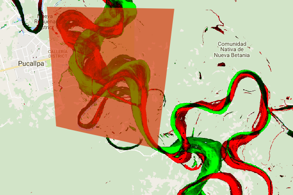
Dans la section "Constants" (Constantes) du code, ajoutez une instruction qui crée une variable définissant le style de la couche. Ce style montre les zones où la présence d'eau de surface a diminué/augmenté en rouge/vert. Les zones où la présence d'eau de surface est relativement inchangée sont indiquées en noir.

Éditeur de code (JavaScript)

var VIS_CHANGE = {
    min:-50,
    max:50,
    palette: ['red', 'black', 'limegreen']
};

À la fin de la section de code "Map Layers" (Calques de carte), ajoutez une instruction qui ajoute un calque à la carte.

Éditeur de code (JavaScript)

Map.setCenter(-74.4557, -8.4289, 11);  // Ucayali River, Peru
Map.addLayer({
  eeObject: change,
  visParams: VIS_CHANGE,
  name: 'occurrence change intensity'
});

Figure 6. Capture d'écran de l'intensité de la variation des eaux de surface pour le fleuve Ucayali près de Pucallpa, une ville de la forêt amazonienne de l'est du Pérou. Le rouge/vert indique une diminution/augmentation de la présence d'eau de surface entre les époques.

Résumer les changements dans une région d'intérêt

Dans cette section, nous allons résumer l'ampleur du changement dans une région d'intérêt spécifique. Pour spécifier une région d'intérêt, cliquez sur l'outil de dessin de polygones, qui fait partie des outils de géométrie. Cela crée un calque "geometry" (géométrie) nommé "geometry" par défaut. Pour modifier le nom, cliquez sur l'icône en forme de roue dentée située à droite du nom du calque. (Notez que vous devrez peut-être placer le curseur sur le nom du calque pour qu'il apparaisse.)

Remplacez le nom du calque par roi (pour la région d'intérêt). Nous pouvons ensuite cliquer sur une série de points sur la carte pour définir une région d'intérêt polygonale.

Figure 7. Capture d'écran du fleuve Ucayali près de Pucallpa, au Pérou, avec une région d'intérêt créée à l'aide de l'outil de dessin de polygones.

Maintenant que notre région d'intérêt est définie et stockée dans une variable, nous pouvons l'utiliser pour calculer un histogramme de l'intensité du changement pour la ROI. Ajoutez le code suivant à la section "Calculations" du script.

Éditeur de code (JavaScript)

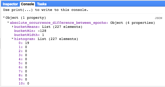
// Calculate a change intensity for the region of interest.
var histogram = change.reduceRegion({
  reducer: ee.Reducer.histogram(),
  geometry: roi,
  scale: 30,
  bestEffort: true,
});
print(histogram);

La première instruction calcule un histogramme des valeurs d'intensité de variation des occurrences dans le ROI, en échantillonnant à une échelle de 30 m. La seconde imprime l'objet résultant dans l'onglet "Console" de l'éditeur de code. Vous pouvez développer l'arborescence des objets pour afficher les valeurs des buckets d'histogramme. Les données numériques sont présentes, mais il existe de meilleures façons de visualiser les résultats.

Figure 8. Résultats de l'onglet "Console" affichant les valeurs d'histogramme de l'intensité de la variation des eaux de surface.

Pour améliorer cela, nous pouvons générer un histogramme à la place. Remplacez l'instruction qui définit l'objet d'histogramme par les instructions suivantes :

Éditeur de code (JavaScript)

// Generate a histogram object and print it to the console tab.
var histogram = ui.Chart.image.histogram({
  image: change,
  region: roi,
  scale: 30,
  minBucketWidth: 10
});
histogram.setOptions({
  title: 'Histogram of surface water change intensity.'
});

Ces instructions créent un objet de graphique d'histogramme, qui remplace l'arborescence d'objets d'histogramme dans l'onglet "Console" par un graphique. La méthode de graphique contient plusieurs arguments, y compris scale qui définit l'échelle spatiale, en mètres, à laquelle la région d'intérêt est échantillonnée, et minBucketWidth qui est utilisé pour contrôler la largeur des buckets d'histogramme.

Figure 9. Résultats de l'onglet "Console", affichant un histogramme de l'intensité de l'évolution des eaux de surface.

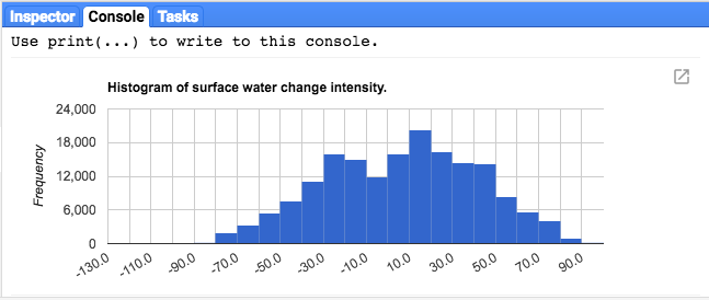
Vous pouvez explorer les valeurs du graphique de manière interactive en plaçant le curseur sur les barres de l'histogramme.

Script final

Le script complet de cette section est listé ci-dessous. Notez que le script inclut des instructions pour définir une géométrie de polygone (roi), qui est comparable à la géométrie que vous avez créée à l'aide des outils de géométrie de l'éditeur de code.

Éditeur de code (JavaScript)

//////////////////////////////////////////////////////////////
// Asset List
//////////////////////////////////////////////////////////////

var gsw = ee.Image('JRC/GSW1_0/GlobalSurfaceWater');
var occurrence = gsw.select('occurrence');
var change = gsw.select("change_abs");
var roi = /* color: 0B4A8B */ee.Geometry.Polygon(
        [[[-74.17213, -8.65569],
          [-74.17419, -8.39222],
          [-74.38362, -8.36980],
          [-74.43031, -8.61293]]]);

//////////////////////////////////////////////////////////////
// Constants
//////////////////////////////////////////////////////////////

var VIS_OCCURRENCE = {
    min:0,
    max:100,
    palette: ['red', 'blue']
};
var VIS_CHANGE = {
    min:-50,
    max:50,
    palette: ['red', 'black', 'limegreen']
};
var VIS_WATER_MASK = {
  palette: ['white', 'black']
};

//////////////////////////////////////////////////////////////
// Calculations
//////////////////////////////////////////////////////////////

// Create a water mask layer, and set the image mask so that non-water areas are transparent.
var water_mask = occurrence.gt(90).mask(1);

// Generate a histogram object and print it to the console tab.
var histogram = ui.Chart.image.histogram({
  image: change,
  region: roi,
  scale: 30,
  minBucketWidth: 10
});
histogram.setOptions({
  title: 'Histogram of surface water change intensity.'
});
print(histogram);

//////////////////////////////////////////////////////////////
// Initialize Map Location
//////////////////////////////////////////////////////////////

// Uncomment one of the following statements to center the map on
// a particular location.
// Map.setCenter(-90.162, 29.8597, 10);   // New Orleans, USA
// Map.setCenter(-114.9774, 31.9254, 10); // Mouth of the Colorado River, Mexico
// Map.setCenter(-111.1871, 37.0963, 11); // Lake Powell, USA
// Map.setCenter(149.412, -35.0789, 11);  // Lake George, Australia
// Map.setCenter(105.26, 11.2134, 9);     // Mekong River Basin, SouthEast Asia
// Map.setCenter(90.6743, 22.7382, 10);   // Meghna River, Bangladesh
// Map.setCenter(81.2714, 16.5079, 11);   // Godavari River Basin Irrigation Project, India
// Map.setCenter(14.7035, 52.0985, 12);   // River Oder, Germany & Poland
// Map.setCenter(-59.1696, -33.8111, 9);  // Buenos Aires, Argentina\
Map.setCenter(-74.4557, -8.4289, 11);  // Ucayali River, Peru

//////////////////////////////////////////////////////////////
// Map Layers
//////////////////////////////////////////////////////////////

Map.addLayer({
  eeObject: water_mask,
  visParams: VIS_WATER_MASK,
  name: '90% occurrence water mask',
  shown: false
});
Map.addLayer({
  eeObject: occurrence.updateMask(occurrence.divide(100)),
  name: "Water Occurrence (1984-2015)",
  visParams: VIS_OCCURRENCE,
  shown: false
});
Map.addLayer({
  eeObject: change,
  visParams: VIS_CHANGE,
  name: 'occurrence change intensity'
});

Dans la section suivante, vous explorerez plus en détail l'évolution de l'eau au fil du temps en travaillant avec la couche de transition de la classe d'eau.